
Most recent TBTK release at the time of writing: v1.1.1
Updated to work with: v2.0.0
In condensed matter physics, the electronic band structure is one of the most commonly used tools for understanding the electronic properties of a material. Here we take a look at how to set up a tight-binding model of graphene and calculate the band structure along paths between certain high symmetry points in the Brillouin zone. We also calculate the density of states (DOS). A basic understanding of band theory is assumed and if further background is required a good starting point is to look at the nearly free electron model, Bloch waves, Bloch’s theorem, and the Brillouin zone.
Physical description
Lattice
Graphene has a hexagonal lattice that can be described using the lattice vectors  ,
,  , and
, and  . We set the lattice constant to
  , which only is meant to reflect the correct order of magnitude. Strictly speaking, only two two-dimensional vectors are required to describe the lattice. However, we have here made the vectors three-dimensional and included a third lattice vector
  that is perpendicular to the lattice to simplify the calculation of the reciprocal lattice vectors. The resulting lattice is shown in the image below.
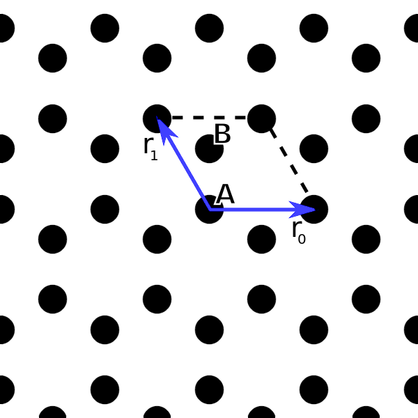
Indicated in the image is also the unit cell and the A and B sublattice sites within the unit cell. We further define
![\[ \begin{aligned} \mathbf{r}_{AB}^{(0)} =& \frac{\mathbf{r}_0 + 2\mathbf{r}_1}{3},\\ \mathbf{r}_{AB}^{(1)} =& -\mathbf{r}_1 + \mathbf{r}_{AB}^{(0)},\\ \mathbf{r}_{AB}^{(2)} =& -\mathbf{r}_0 - \mathbf{r}_1 + \mathbf{r}_{AB}^{(0)}, \end{aligned} \]](http://second-tech.com/wordpress/wp-content/ql-cache/quicklatex.com-78cf9c0b57f89e789f9743d503fa0706_l3.png "Rendered by QuickLaTeX.com")
which can be verified to be the vector from A to its three nearest neighbor B sites.
Brillouin zone
The reciprocal lattice vectors can now be calculated using
![\[ \begin{aligned} \mathbf{k}_0 =& \frac{2\pi \mathbf{r}_1\times\mathbf{r}_2}{\mathbf{r}_0\cdot\mathbf{r}_1\times\mathbf{r}_2},\\ \mathbf{k}_1 =& \frac{2\pi \mathbf{r}_2\times\mathbf{r}_0}{\mathbf{r}_1\cdot\mathbf{r}_2\times\mathbf{r}_0},\\ \mathbf{k}_2 =& \frac{2\pi\mathbf{r}_0\times\mathbf{r}_1}{\mathbf{r}_2\cdot\mathbf{r}_0\times\mathbf{r}_1}. \end{aligned} \]](http://second-tech.com/wordpress/wp-content/ql-cache/quicklatex.com-e9ec406b51d6e8a5e27c358752729d69_l3.png "Rendered by QuickLaTeX.com")
Here  just like is related to the z-direction and will be dropped from here on. The two remaining reciprocal lattice vectors
  and
and  defines the reciprocal lattice of interest to us. Below the reciprocal lattice is shown.
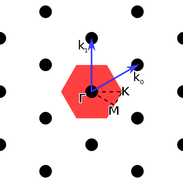
In the the image above we have also indicated the first Brillouin zone in red, and outlined the path  along which the band structure will be calculated. The high symmetry points can be verified to be given by
![\[ \begin{aligned} \mathbf{\Gamma} =& (0, 0, 0),\\ \mathbf{M} =& (\frac{\pi}{a}, \frac{-\pi}{\sqrt{3}a}, 0),\\ \mathbf{K} =& (\frac{4\pi}{3a}, 0, 0). \end{aligned} \]](http://second-tech.com/wordpress/wp-content/ql-cache/quicklatex.com-b5445661f8865929eb0d02a1b38f213e_l3.png "Rendered by QuickLaTeX.com")
Hamiltonian
We will use a simple tight-binding model of graphene of the form
![\[ H = -t\sum_{\mathbf{i}\delta}c_{\mathbf{i},A}^{\dagger}c_{\mathbf{i}+\boldsymbol{\delta},B} + H.c. \]](http://second-tech.com/wordpress/wp-content/ql-cache/quicklatex.com-9c89065579ce76668ed7da6d9e2c24a3_l3.png "Rendered by QuickLaTeX.com")
Here  is a hopping amplitude connecting nearest neighbor sites which we take to be
  (again, only correct up to order of magnitude). The index
  runs over the unit cells, while
  takes on the three values that makes
  the nearest neighbor of
  .
.
Because of translation invariance, it is possible to transform the expression above to a simple expression in reciprocal space. To do so we write
![\[ \begin{aligned} c_{\mathbf{i},A} =& \frac{1}{\sqrt{N}}\sum_{\mathbf{k}}c_{\mathbf{k},A}e^{ik\cdot \mathbf{R}_{\mathbf{i}}},\\ c_{\mathbf{i}+\boldsymbol\delta},B} =& \frac{1}{\sqrt{N}}\sum_{\mathbf{k}}c_{\mathbf{k},B}e^{i\mathbf{k}\cdot \left(\mathbf{R}_{\mathbf{i}} + \mathbf{r}_{\boldsymbol\delta}\right)}. \end{aligned} \]](http://second-tech.com/wordpress/wp-content/ql-cache/quicklatex.com-09bdc2b0dc0d16dbb74d1521382c2074_l3.png "Rendered by QuickLaTeX.com")
Here  is the position of the A atom in unit cell , while
  .1
.1
Inserting this into the expression above we get
![\[ \begin{aligned} H =& \frac{-t}{N}\sum_{i\mathbf{k}\mathbf{k}'\boldsymbol{\delta}}c_{\mathbf{k},A}^{\dagger}c_{\mathbf{k}',B}e^{-i\mathbf{k}\cdot \mathbf{R}_{\mathbf{i}}}e^{i\mathbf{k}'\cdot\left(\mathbf{R}_{\mathbf{i}} + \mathbf{r}_{\boldsymbol{\delta}}\right)} + H.c\\ =& -t\sum_{\mathbf{k}\boldsymbol{\delta}}c_{\mathbf{k},A}^{\dagger}c_{\mathbf{k},B}e^{i\mathbf{k}\cdot \mathbf{r}_{\boldsymbol{\delta}}} + H.c\\ =& -t\sum_{\mathbf{k}}c_{\mathbf{k},A}^{\dagger}c_{\mathbf{k},B}\left(e^{i\mathbf{k}\cdot\mathbf{r}_{AB}^{(0)}} + e^{i\mathbf{k}\cdot\mathbf{r}_{AB}^{(1)}} + e^{i\mathbf{k}\cdot\mathbf{r}_{AB}^{(2)}}\right) + H.c. \end{aligned} \]](http://second-tech.com/wordpress/wp-content/ql-cache/quicklatex.com-0e966222b1b37543d4062c651033c281_l3.png "Rendered by QuickLaTeX.com")
In the second line we have summed over and used the delta function property of  to eliminat
  , while in the last line we have made the sum over explicit.
Implementation
Parameters
We are now ready to implement the calculation using TBTK. To do so, we begin by specifying the parameters to be used in the calculation
//Set the natural units for this calculation.
UnitHandler::setScales({
        "1 rad", "1 C", "1 pcs", "1 eV",
        "1 Ao", "1 K", "1 s"
});

//Define parameters.
double t = 3;   //eV
double a = 2.5; //Ångström
unsigned int BRILLOUIN_ZONE_RESOLUTION = 1000;
vector<unsigned int> numMeshPoints = {
    BRILLOUIN_ZONE_RESOLUTION,
    BRILLOUIN_ZONE_RESOLUTION
};
const int K_POINTS_PER_PATH = 100;
const double ENERGY_LOWER_BOUND = -10;
const double ENERGY_UPPER_BOUND = 10;
const int ENERGY_RESOLUTION = 1000;
In lines 2-5, we specify what units that dimensionful parameters should be understood in terms of. For our purposes here, this means that energies and distances are measured in electron Volts (eV) and Ångström (Ao), respectively.
We next specify the value for and  as given in the physical description above. The value ‘BRILLOUIN_ZONE_RESOLUTION’ determines the number of subintervals each of the reciprocal lattice vectors is divided into when generating a mesh for the Brillouin zone. ‘numMeshPoints’ combine this information into a vector. Similarly, ‘K_POINTS_PER_PATH’ determines the number of k-points to use along each of the paths
  ,
,  , and
, and  when calculating the band structure. Finally, the energy window that is used to calculate the DOS is specified in the three last lines.
Real and reciprocal lattice
The lattice vectors  ,
,  , and
, and  are now defined as follows.
Vector3d r[3];
r[0] = Vector3d({a,     0,              0});
r[1] = Vector3d({-a/2,  a*sqrt(3)/2,    0});
r[2] = Vector3d({0,     0,              a});
The nearest neighbor vectors  ,
,  , and
, and  are similarly defined using
Vector3d r_AB[3];
r_AB[0] = (r[0] + 2*r[1])/3.;
r_AB[1] = -r[1] + r_AB[0];
r_AB[2] = -r[0] - r[1] + r_AB[0];
Next, the reciprocal lattice vectors are calculated using the expressions at the beginning of the Brillouin zone section.
Vector3d k[3];
for(unsigned int n = 0; n < 3; n++){
    k[n] = 2*M_PI*r[(n+1)%3]*r[(n+2)%3]/(
        Vector3d::dotProduct(
            r[n],
            r[(n+1)%3]*r[(n+2)%3]
        )
    );
}
Note that here ‘*’ indicates the cross product, while the scalar product between u and v is calculated using Vector3d::dotProduct(u, v).
Having defined the lattice vectors, we can now construct a Brillouin zone.
BrillouinZone brillouinZone(
    {
        {k[0].x, k[0].y},
        {k[1].x, k[1].y}
    },
    SpacePartition::MeshType::Nodal
);
Here the first argument is a list of lattice vectors, while the second argument specifies the type of mesh that is going to be associated with this Brillouin zone. SpacePartition::MeshType::Nodal means that when the Brillouin zone is divided into small parallelograms, the mesh points will lie on the corners of these parallelograms. If SpacePartition::MeshType::Interior is used instead, the mesh points will lie in the middle of the parallelograms.
Having constructed a Brillouin zone, we finally generate a mesh by passing the number of segments to divide each reciprocal lattice vector to the following function.
vector<vector<double>> mesh
    = brillouinZone.getMinorMesh(
        numMeshPoints
    );
Set up the model
The model is set up using the following code.
Model model;
for(unsigned int n = 0; n < mesh.size(); n++){
    //Get Index representation of the current
    //k-point.
    Index kIndex = brillouinZone.getMinorCellIndex(
        mesh[n],
        numMeshPoints
    );

    //Calculate the matrix element.
    Vector3d k({mesh[n][0], mesh[n][1], 0});
    complex<double> h_01 = -t*(
        exp(
            -i*Vector3d::dotProduct(
                k,
                r_AB[0]
            )
        )
        + exp(
            -i*Vector3d::dotProduct(
                k,
                r_AB[1]
            )
        )
        + exp(
            -i*Vector3d::dotProduct(
                k,
                r_AB[2]
            )
        )
    );

    //Add the matrix element to the model.
    model << HoppingAmplitude(
        h_01,
        {kIndex[0], kIndex[1], 0},
        {kIndex[0], kIndex[1], 1}
    ) + HC;
}
model.construct();
Here the loop runs over each lattice point in the mesh. To understand line 4-7, we first note that the mesh contains k-points of the form  with real numbers
  and
and  . However, to specify a model, we need discrete indices with integer-valued subindices to label the points. Think of this as each k value being of the form
  , where is a real-valued vector while is an integer-valued vector that indexes the different k-points. The BrillouinZone solves this problem for us by automatically providing a mapping from continuous indices to discrete indices. Given a real index in the first Brillouin zone and information about the number of subdivisions of the lattice vectors, brillouinZone.getMinorCellIndex() finds the closest discrete point and returns its Index representation. This index can then be used to refer to the k-point whenever an Index object is required.
In line 10, the mesh point is converted to a Vector3d object that is then used in lines 11-30 to calculate the matrix element we derived in the section about the Hamiltonian. The matrix element, together with its Hermitian conjugate, is then fed to the model in lines 33-37. Here we construct the full index for the model by combining the integer kIndex[0] and kIndex[1] values, together with the sublattice index, into an index structure of the form {kx, ky, sublattice}. A zero in the sublattice index refers to an A site, while one refers to a B site. Finally, the model is constructed in line 39.
Selecting solver
We are now ready to solve the model and will use diagonalization to do so. In this case, we have a problem that is block-diagonal in the k-index. For this reason, we will use the solver Solver::BlockDiagonalizer that can take advantage of this block structure. To set up and run the diagonalization we write
Solver::BlockDiagonalizer solver;
solver.setModel(model);
solver.run();
We then set up the corresponding property extractor and configure the energy window using
PropertyExtractor::BlockDiagonalizer
    propertyExtractor(solver);
propertyExtractor.setEnergyWindow(
    ENERGY_LOWER_BOUND,
    ENERGY_UPPER_BOUND,
    ENERGY_RESOLUTION
);
Extracting the DOS
Extracting, smoothing, and plotting the DOS is now done as follows.
//Calculate the density of states (DOS).
Property::DOS dos
    = propertyExtractor.calculateDOS();

//Smooth the DOS.
const double SMOOTHING_SIGMA = 0.03;
const unsigned int SMOOTHING_WINDOW = 51;
dos = Smooth::gaussian(
    dos,
    SMOOTHING_SIGMA,
    SMOOTHING_WINDOW
);

//Plot the DOS.
Plotter plotter;
plotter.plot(dos);
plotter.save("figures/DOS.png");
Extract the band structure
We are now ready to calculate the band structure. To do so, we begin by defining the high symmetry points
Vector3d Gamma({0,        0,                 0});
Vector3d M({M_PI/a,       -M_PI/(sqrt(3)*a), 0});
Vector3d K({4*M_PI/(3*a), 0,                 0});
These are then packed in pairs to define the three paths , , and
vector<vector<Vector3d>> paths = {
    {Gamma, M},
    {M, K},
    {K, Gamma}
};
We now loop over each of the three paths and calculate the band structure at each k-point along these paths.
Array<double> bandStructure(
    {2, 3*K_POINTS_PER_PATH},
    0
);
Range interpolator(0, 1, K_POINTS_PER_PATH);
for(unsigned int p = 0; p < 3; p++){
    //Select the start and endpoints for the
    //current path.
    Vector3d startPoint = paths[p][0];
    Vector3d endPoint = paths[p][1];

    //Loop over a single path.
    for(
        unsigned int n = 0;
        n < K_POINTS_PER_PATH;
        n++
    ){
        //Interpolate between the paths start
        //and end point.
        Vector3d k = (
            interpolator[n]*endPoint
            + (1 - interpolator[n])*startPoint
        );

        //Get the Index representation of the
        //current k-point.
        Index kIndex = brillouinZone.getMinorCellIndex(
            {k.x, k.y},
            numMeshPoints
        );

        //Extract the eigenvalues for the
        //current k-point.
        bandStructure[
            {0, n+p*K_POINTS_PER_PATH}
        ] = propertyExtractor.getEigenValue(
            kIndex,
            0
        );
        bandStructure[
            {1, n+p*K_POINTS_PER_PATH}
        ] = propertyExtractor.getEigenValue(
            kIndex,
            1
        );
    }
}
Here we first set up the array ‘bandStructure’ that is to contain the band structure with two eigenvalues per k-point. The variable ‘interpolator’ is then defined, which is an array of values from 0 to 1 that will be used to interpolate between the paths start and endpoints. In lines 9 and 10 we then select the start and endpoints for the current path, and the loop over this path begins in line 13.
In lines 20-23, we calculate an interpolated k-point value between the first and last points in the given path. Similarly, as when setting up the model, we then request the Index that corresponds to the given k-point. Having obtained this Index, we extract the lowest eigenvalue for the corresponding block in lines 34-39 and store it in the array ‘bandStructure’. Similarly, the highest eigenvalue is obtained for the same block in lines 40-45.
Next, we calculate the maximum and minimum value of the band structure along the calculated paths. We do this to allow for drawing vertical lines of the correct height at the M and K points when plotting the data.
double min = bandStructure[{0, 0}];
double max = bandStructure[{1, 0}];
for(
    unsigned int n = 0;
    n < 3*K_POINTS_PER_PATH; n++ ){ if(min > bandStructure[{0, n}])
        min = bandStructure[{0, n}];
    if(max < bandStructure[{1, n}])
        max = bandStructure[{1, n}];
}
Finally, we plot the band structure.
plotter.clear();
plotter.setLabelX("k");
plotter.setLabelY("Energy");
plotter.plot(
    bandStructure.getSlice({0, _a_}),
    {{"color", "black"}}
);
plotter.plot(
    bandStructure.getSlice({1, _a_}),
    {{"color", "black"}}
);
plotter.plot(
    {K_POINTS_PER_PATH, K_POINTS_PER_PATH},
    {min, max},
    {{"color", "black"}}
);
plotter.plot(
    {2*K_POINTS_PER_PATH, 2*K_POINTS_PER_PATH},
    {min, max}
    {{"color", "black"}}
);
plotter.save("figures/BandStructure.png ");
Here the ‘_a_’ flag in the call to bandStructure.getSlice({0, _a_}, {{“color”, “black”}}) on line 5 (and 6) is a wildcard. It indicates that we want to get a new array that contains all the elements of the original array that has a zero in the first index and an arbitrary index in the second. ‘a’ stands for ‘all’.
Results
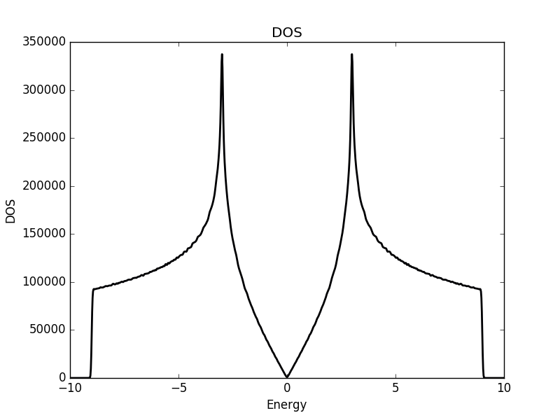
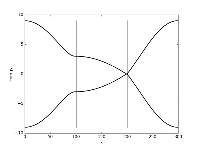
Below the results are shown. The DOS is characteristically v-shaped around  and is peaked 1/3 of the way to the band edge. In the band structure, we can see the Dirac cone at the K-point (the second vertical line). The low density of states at can be understood as a consequence of the small number of k-points around the K-point for which the energy is close to zero. The cone has a finite slope, and therefore only a single k-point is at (one more point is at the
  -point, which we have not considered here but which is at another corner of the Brillouin zone). Compare this with the flat region at the M-point (first vertical line), which results in a significant amount of k-points with roughly the same energy. This flat region is responsible for the strong peaks in the DOS.
DOS
Band structure
Full code
The full code is available in src/main.cpp in the project 2019_07_05 of the Second Tech code package. See the README for instructions on how to build and run.
![\[ \frac{df(x)}{dx} = \lim_{\Delta x\rightarrow 0}\frac{f(x + \Delta x) - f(x - \Delta x)}{2\Delta x}. \]](http://second-tech.com/wordpress/wp-content/ql-cache/quicklatex.com-4e5b7b4edc4b258a9f1651b32a05d14d_l3.png "Rendered by QuickLaTeX.com")
![\[ \frac{df(x)}{dx} \approx \frac{f(x + \Delta x) - f(x - \Delta x)}{2\Delta x}, \]](http://second-tech.com/wordpress/wp-content/ql-cache/quicklatex.com-6eaf348106089f6af8d0b1e511a86fcb_l3.png "Rendered by QuickLaTeX.com")
 .
. for integer
  . Moreover, since the finite difference approximation should be understood to be valid for each of these points, it really is a set of linear equations of the form
![\[ \begin{aligned} ... & ...\\ \frac{df(x_n)}{dx} &\approx \frac{f(x_{n+1}) - f(x_{n-1})}{2\Delta x},\\ \frac{df(x_{n+1})}{dx} &\approx \frac{f(x_{n+2}) - f(x_n)}{2\Delta x},\\ ... & ... \end{aligned} \]](http://second-tech.com/wordpress/wp-content/ql-cache/quicklatex.com-bc3b6122c3f8797d780bfa466c093aa6_l3.png "Rendered by QuickLaTeX.com")
![\[\left[\begin{array}{c} ...\\ \frac{df(x_n)}{dx}\\ \frac{df(x_{n+1})}{dx}\\ ... \end{array}\right] \approx D^{(1)}\left[\begin{array}{c} ...\\ f(x_n)\\ f(x_{n+1})\\ ... \end{array}\right], \]](http://second-tech.com/wordpress/wp-content/ql-cache/quicklatex.com-c3f75bb9206cd612679e2c3e39cf8a1f_l3.png "Rendered by QuickLaTeX.com")
![\[ D^{(1)} = \frac{1}{2\Delta x}\left[\begin{array}{cccccc} ... & ... & ... & ... & ... & ...\\ ... & -1 & 0 & 1 & 0 & ...\\ ... & 0 & -1 & 0 & 1 & ...\\ ... & ... & ... & ... & ... & ... \end{array}\right].\]](http://second-tech.com/wordpress/wp-content/ql-cache/quicklatex.com-d12f8ad72b2c77d0dd06ce24371e9770_l3.png "Rendered by QuickLaTeX.com")
 and
and  appear right below and above the diagonal, respectively.
 for some finite
  . The matrix therefore necessarily have to be truncated, which means that the first and last row in fact corresponds to
![\[\begin{aligned} \frac{df(x_{0})}{dx} &\approx \frac{f(x_1) - 0}{2\Delta x},\\ \frac{df(x_{N-1})}{dx} &\approx \frac{0 - f(x_{N-2})}{2\Delta x}. \end{aligned}\]](http://second-tech.com/wordpress/wp-content/ql-cache/quicklatex.com-4537d9e33c519464c7cf3fee10af2df9_l3.png "Rendered by QuickLaTeX.com")
 . Other boundary conditions can be added back into the formulation, but for simplicity we will consider these boundary conditions here.
![\[\begin{aligned} \frac{df(x)}{dx} &= \lim_{\Delta x \rightarrow 0}\frac{f(x + \Delta x) - f(x)}{\Delta x},\\ \frac{df(x)}{dx} &= \lim_{\Delta x \rightarrow 0}\frac{f(x + \Delta x) - f(x - \Delta x)}{2\Delta x},\\ \frac{df(x)}{dx} &= \lim_{\Delta x \rightarrow 0}\frac{f(x) - f(x - \Delta x)}{\Delta x}. \end{aligned}\]](http://second-tech.com/wordpress/wp-content/ql-cache/quicklatex.com-ddc79e8e373525ac60051f252a75c23d_l3.png "Rendered by QuickLaTeX.com")
 instead of
  . Moreover, the two matrices also have the -1 and 1 off-diagonal entries moved onto the diagonal, respectively. This leads to a different type of boundary conditions once the matrix is truncated. However, here we will not be interested in the finite difference expression for the first derivative directly. Rather, the forward and backward differences are of interest to us since they allow us to arrive at a simple expression for the second derivative.
![\[ \frac{d^2f(x)}{dx^2} = \lim_{\Delta x \rightarrow 0}\frac{\frac{df(x + \frac{\Delta x}{2})}{dx} - \frac{df(x - \frac{\Delta x}{2})}{dx}}{\Delta x}. \]](http://second-tech.com/wordpress/wp-content/ql-cache/quicklatex.com-965f4a4865286f63971c9b12d3b1f7b1_l3.png "Rendered by QuickLaTeX.com")
 , or as the forward difference at
  . Similarly the second term can be understood as either the centered difference at
  , or as the backward difference at
  . Plugging in the forward and backward differences and removing the limit, we get
![\[ \frac{d^2f(x)}{dx^2} \approx \frac{f(x + \Delta x) - 2f(x) + f(x - \Delta x)}{\Delta x^2}. \]](http://second-tech.com/wordpress/wp-content/ql-cache/quicklatex.com-15e7c67213cb2d1677be621684170067_l3.png "Rendered by QuickLaTeX.com")
![\[\left[\begin{array}{c} ...\\ \frac{d^2f(x_n)}{dx^2}\\ \frac{d^2f(x_{n+1})}{dx^2}\\ ... \end{array}\right] \approx D^{(2)}\left[\begin{array}{c} ...\\ f(x_n)\\ f(x_{n+1})\\ ... \end{array}\right], \]](http://second-tech.com/wordpress/wp-content/ql-cache/quicklatex.com-670d76e00be6e69d68f6eba8f70e4e69_l3.png "Rendered by QuickLaTeX.com")
![\[ D^{(2)} = \frac{1}{\Delta x^2}\left[\begin{array}{cccccc} ... & ... & ... & ... & ... & ...\\ ... & 1 & -2 & 1 & 0 & ...\\ ... & 0 & 1 & -2 & 1 & ...\\ ... & ... & ... & ... & ... & ... \end{array}\right].\]](http://second-tech.com/wordpress/wp-content/ql-cache/quicklatex.com-8071a3931503033ac032e660a669dc01_l3.png "Rendered by QuickLaTeX.com")
![\[ H\Psi(x) = \left(\frac{-\hbar^2}{2m}\frac{d^2}{dx^2} + V(x)\right)\Psi(x). \]](http://second-tech.com/wordpress/wp-content/ql-cache/quicklatex.com-a26d3ce344d8035e01c632cf52752fb1_l3.png "Rendered by QuickLaTeX.com")
 is defined on a discrete lattice, the potential
  becomes a diagonal matrix
  with
with  along the diagonal. Using this together with the discretized approximation of the second derivative derived above, the discretized Hamiltonian becomes
![\[ H_{D} = \frac{-\hbar^2}{2m}D^{(2)} + V. \]](http://second-tech.com/wordpress/wp-content/ql-cache/quicklatex.com-7537870d15efeaed400317781715d26b_l3.png "Rendered by QuickLaTeX.com")
![\[ H_{sq} = \sum_{\mathbf{i}\mathbf{j}}a_{\mathbf{i}\mathbf{j}}c_{\mathbf{i}}^{\dagger}c_{\mathbf{j}}. \]](http://second-tech.com/wordpress/wp-content/ql-cache/quicklatex.com-565fa947c6d4c41105c9d438ab3a7ff7_l3.png "Rendered by QuickLaTeX.com")
 . That is,
  can be understood as generalized row and column indices, respectively.
 and
and  , while for the first off-diagonals we find
  . Separating the two diagonal terms, we can implement the model specification in TBTK as follows.
 , while the potential term has been added by passing the callback *potentialCallback* as the first parameter to the HoppingAmplitude.
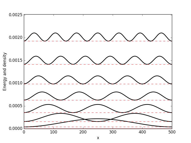
 . While it from an algorithmic standpoint is very useful to consider
  to be a vector with a linear index
  , it is from an intuitive point of view more natural to work with states using a notation such as
  . In TBTK notation where both coordinates and indices necessarily are discrete, this can be encoded as {x, y, s}.
![\[ \textrm{HoppingAmplitude(-t, \{0, 0\}, \{0, 1\})}, \]](http://second-tech.com/wordpress/wp-content/ql-cache/quicklatex.com-7b9e00db9daf6d1ecb5a6619d2b99e2e_l3.png "Rendered by QuickLaTeX.com")
![\[ \langle\Psi_{\{0, 0\}}|H|\Psi_{\{0, 1\}}\rangle = -t, \]](http://second-tech.com/wordpress/wp-content/ql-cache/quicklatex.com-489bfef6c15156e2fbc9509e3731ab25_l3.png "Rendered by QuickLaTeX.com")
![\[ \langle\Psi_{0}|H|\Psi_{1}\rangle = -t. \]](http://second-tech.com/wordpress/wp-content/ql-cache/quicklatex.com-29c3def86aa25f5f1f76918a08a33d33_l3.png "Rendered by QuickLaTeX.com")
![\[ H = -t\sum_{\langle ij\rangle}c_{i}^{\dagger}c_{j}, \]](http://second-tech.com/wordpress/wp-content/ql-cache/quicklatex.com-8192fbef0d654403e8bd881d74741a3a_l3.png "Rendered by QuickLaTeX.com")
 and outer radius
  . Here
  denotes summation over nearest neighbors and the Hamiltonian can be considered to be the (square lattice) discretized version of the Schrödinger equation with
![\[\begin{aligned} H_{S} &= \frac{-\hbar^2}{2m}\left(\frac{\partial^2}{\partial x^2} + \frac{\partial^2}{\partial y^2}\right) + V(x,y)\\ &= \frac{-\hbar^2}{2m}\left(\frac{1}{r}\frac{\partial}{\partial r}\left(r\frac{\partial}{\partial r}\right) + \frac{1}{r^2}\frac{\partial^2}{\partial \theta^2}\right) + V(r, \theta), \end{aligned}\]](http://second-tech.com/wordpress/wp-content/ql-cache/quicklatex.com-792d9a388f86a4b5574a9d21ca16cb5d_l3.png "Rendered by QuickLaTeX.com")
 and
and  .
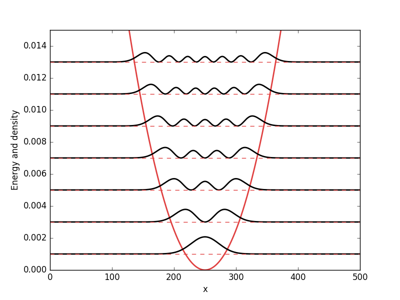
. grid. The fourth and fifth parameter defines the outer and inner radius of the annulus and we also set
  . The last parameter is used to indicate for which state we are going to calculate the energy and probability density.
 from the center of the grid is then calculated and true is returned if
  .
.
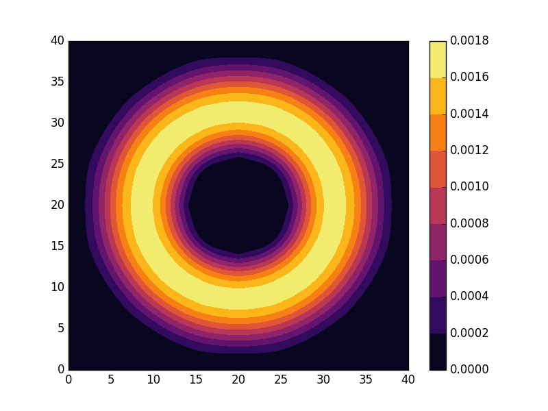


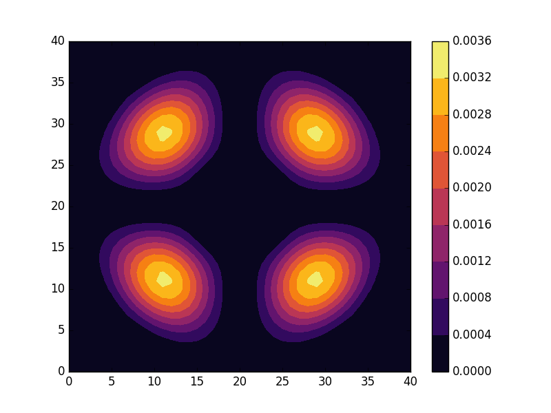


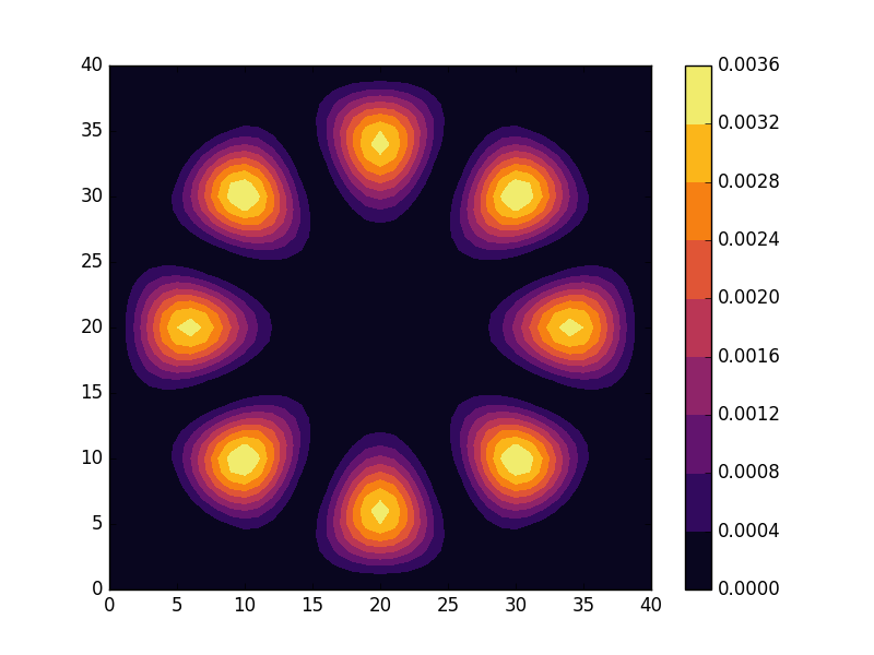


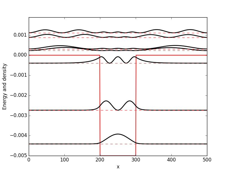
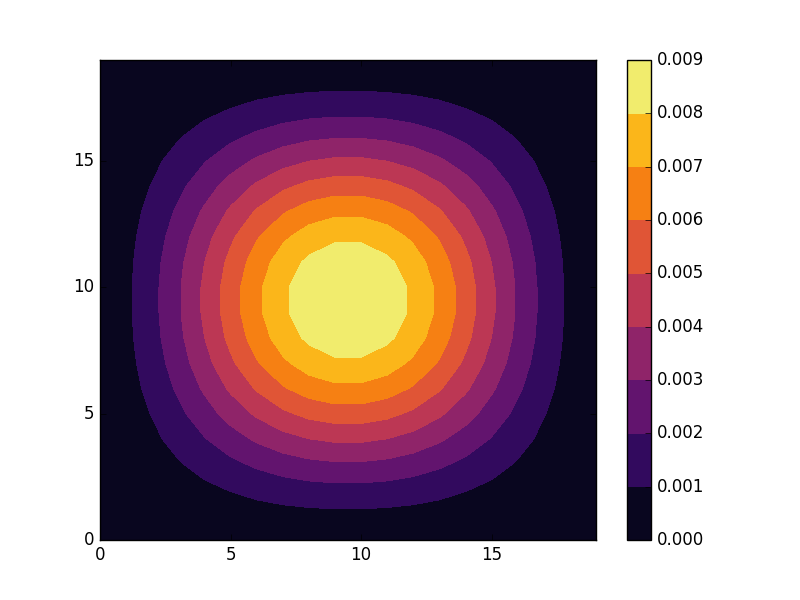
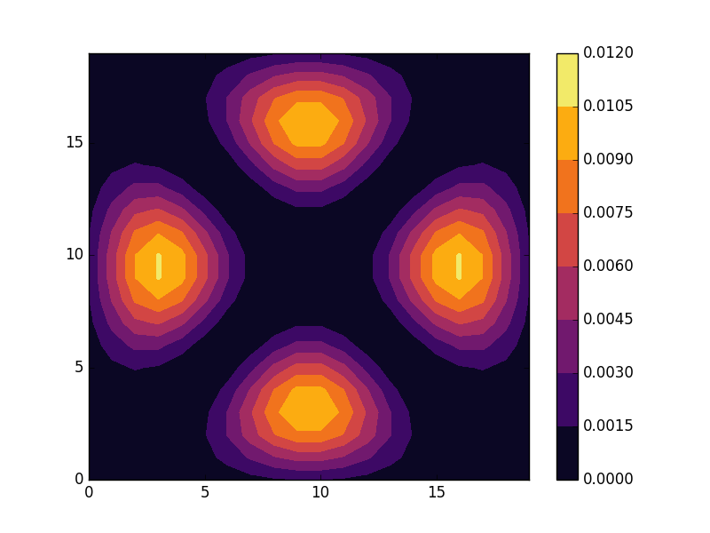
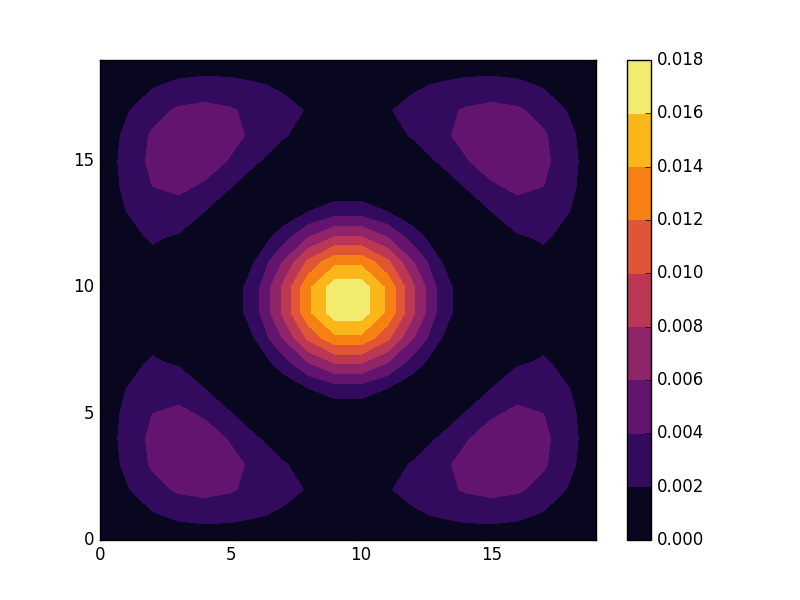
 can be seen to be solved by a function of the form
![\[ f_{n,m}(r, \theta) = f_{n}(r)e^{im\theta}. \]](http://second-tech.com/wordpress/wp-content/ql-cache/quicklatex.com-57f089d025846d33510057ced248434a_l3.png "Rendered by QuickLaTeX.com")
 . Moreover, it can be verified by application of
  to
to  that
that  and
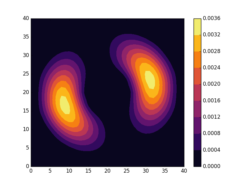
and  are solutions with the same energy. In the continuous case we therefore expect non-degenerate eigenvalues for
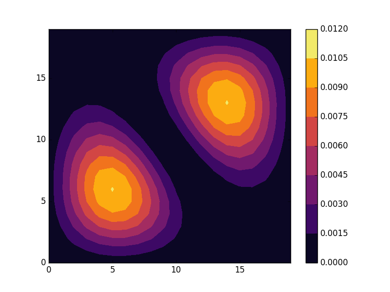
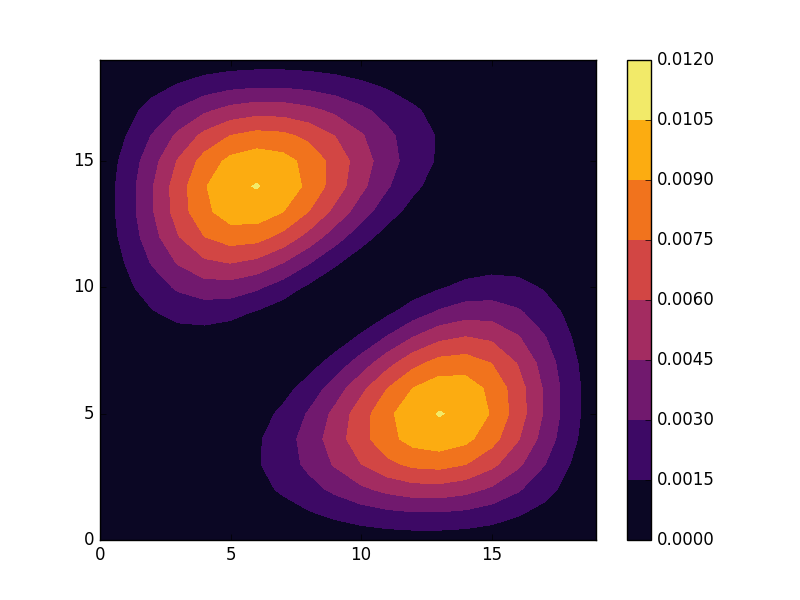
  and doubly degenerate eigenvalues for
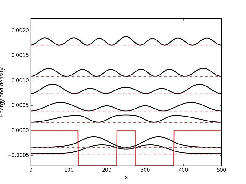
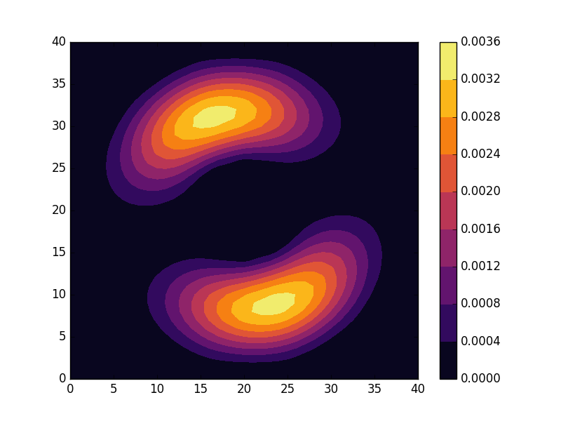
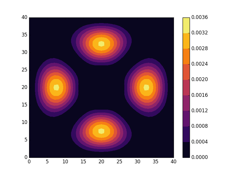
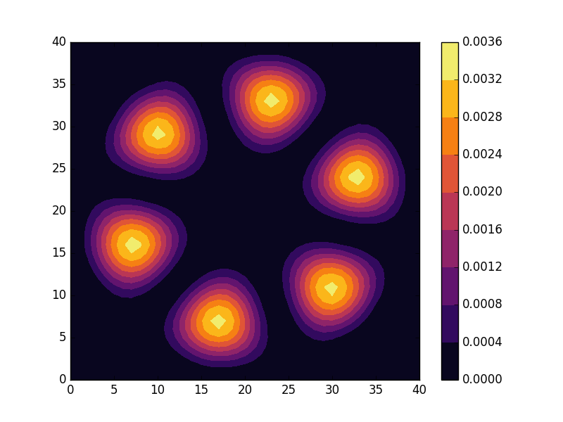
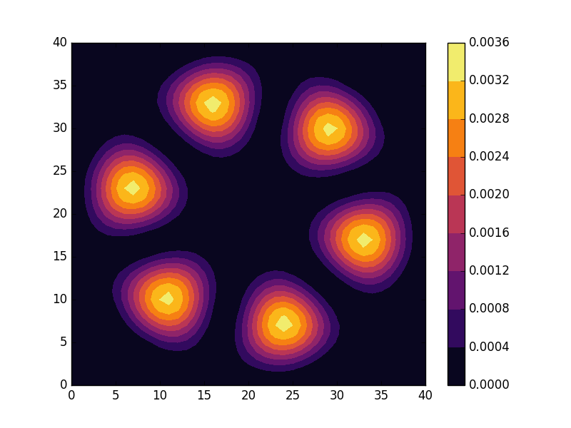
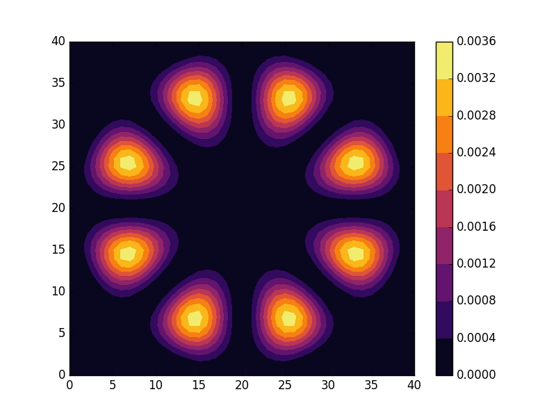
  . For the radial solutions we can further expect a set of increasingly oscillating functions with increasing
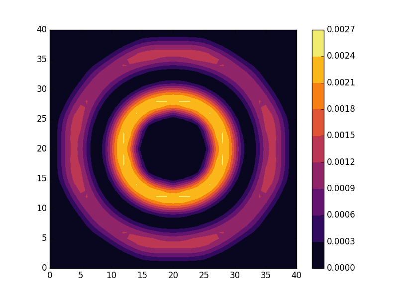
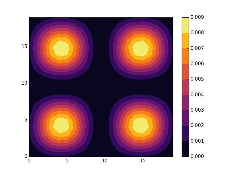
  direction. After state 8 it is no longer energetically favorable to keep increasing the angular wave number, but instead the next energy state is found by once again returning to the non-degenerate case
  , but to increase the radial wave number by one. This is then followed by another set of degenerate states with two radial oscillations and
  .
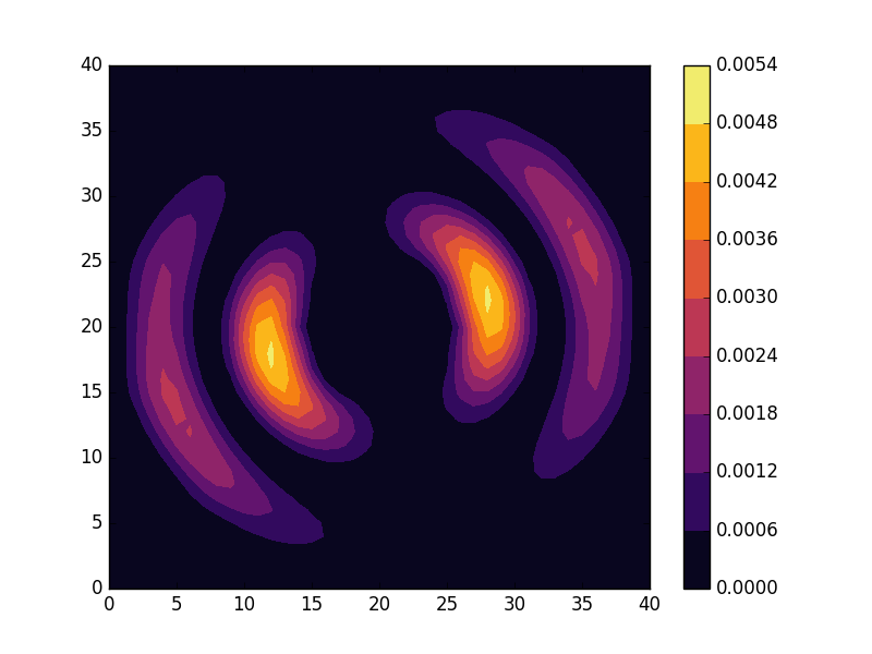
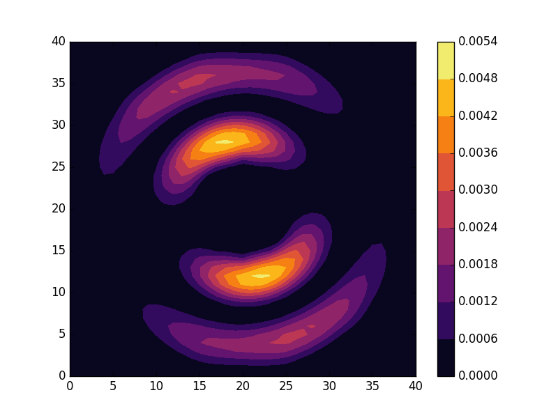
. actually is a constant function of
 ![\[ &\frac{1}{\sqrt{2}}\left(f_{n,m}(r, \theta) + f_{n,-m}(r, \theta)\right) = \sqrt{2}f_{n}(r)\cos(im\theta) \]](http://second-tech.com/wordpress/wp-content/ql-cache/quicklatex.com-1784965f8d2ceacd7e1c3e5026aa796a_l3.png "Rendered by QuickLaTeX.com")
![\[ &\frac{1}{\sqrt{2}}\left(f_{n,m}(r, \theta) + f_{n,-m}(r, \theta)\right) = \sqrt{2}if_{n}(r)\sin(im\theta) \]](http://second-tech.com/wordpress/wp-content/ql-cache/quicklatex.com-8bda533be7e972840f96ec5a69e40f3c_l3.png "Rendered by QuickLaTeX.com")
![\[ H = -t\sum_{\langle ij\rangle}c_{i}^{\dagger}c_{j}. \]](http://second-tech.com/wordpress/wp-content/ql-cache/quicklatex.com-a64258768b7c05fa80ec3c7fb102241a_l3.png "Rendered by QuickLaTeX.com")
 can either be viewed as the simplest example of a two-dimensional tight-binding model, or as a discretized version of the two-dimensional Schrödinger equation
![\[ H_{S} = \frac{-\hbar^2}{2m}\left(\frac{\partial^2}{\partial x^2} + \frac{\partial^2}{\partial y^2}\right) + V(x,y), \]](http://second-tech.com/wordpress/wp-content/ql-cache/quicklatex.com-b47e4a87d5e5d3e769120d4aefe64429_l3.png "Rendered by QuickLaTeX.com")
 . We therefore begin by introducing the following parameters.
![\[\begin{aligned} -t&\left(c_{(x+1,y)}^{\dagger}c_{(x,y)} + c_{(x-1,y)}^{\dagger}c_{(x,y)}\right.\\ &+\left.c_{(x,y+1)}^{\dagger}c_{(x,y)} + c_{(x,y-1)}^{\dagger}c_{(x,y)}\right). \end{aligned}\]](http://second-tech.com/wordpress/wp-content/ql-cache/quicklatex.com-1477295d3655ca6b13ba5e674468ec78_l3.png "Rendered by QuickLaTeX.com")
![\[ -t\left(c_{(x+1,y)}^{\dagger}c_{(x,y)} + c_{(x,y+1)}^{\dagger}c_{(x,y)}\right) + H.c. \]](http://second-tech.com/wordpress/wp-content/ql-cache/quicklatex.com-5de92b1ad2f4a414504749e3e5eca899_l3.png "Rendered by QuickLaTeX.com")
 is the Hermitian conjugate of
  .
.![\[ E \in \{-3.9553, -3.8881, -3.82229, -3.7796\}. \]](http://second-tech.com/wordpress/wp-content/ql-cache/quicklatex.com-24afc190a1c9e903fd516bea9973d95a_l3.png "Rendered by QuickLaTeX.com")
![\[ (m, n) \in \{(1, 1), (2, 1), (1, 2), (2, 2), (3, 1), (1, 3)\}. \]](http://second-tech.com/wordpress/wp-content/ql-cache/quicklatex.com-f60ccc179807430b166048decfef82bf_l3.png "Rendered by QuickLaTeX.com")
![\[ H_{1D} &= -2t\sum_{k_x}\cos(k_x)c_{k_x}^{\dagger}c_{k_x}, \]](http://second-tech.com/wordpress/wp-content/ql-cache/quicklatex.com-5b5b743722b34882e80f324001af702c_l3.png "Rendered by QuickLaTeX.com")
![[-\pi, \pi]](http://second-tech.com/wordpress/wp-content/ql-cache/quicklatex.com-80a7d8bc972a86dd439cfc2467235120_l3.png "Rendered by QuickLaTeX.com") .
.![\[ H_{2D} &= -2t\sum_{k_x,k_y}\left(\cos(k_x) + \cos(k_y)\right)c_{\mathbf{k}}^{\dagger}c_{\mathbf{k}}, \]](http://second-tech.com/wordpress/wp-content/ql-cache/quicklatex.com-699d3420c043827aa34a51af1f716556_l3.png "Rendered by QuickLaTeX.com")
 .
. grid.
grid.![\[ H_{3D} &= -2t\sum_{k_x,k_y,k_z}\left(\cos(k_x) + \cos(k_y) + \cos(k_z)\right)c_{\mathbf{k}}^{\dagger}c_{\mathbf{k}}, \]](http://second-tech.com/wordpress/wp-content/ql-cache/quicklatex.com-8597a453c2ae05fb8a8b9b3331f33d82_l3.png "Rendered by QuickLaTeX.com")
 .
. grid.
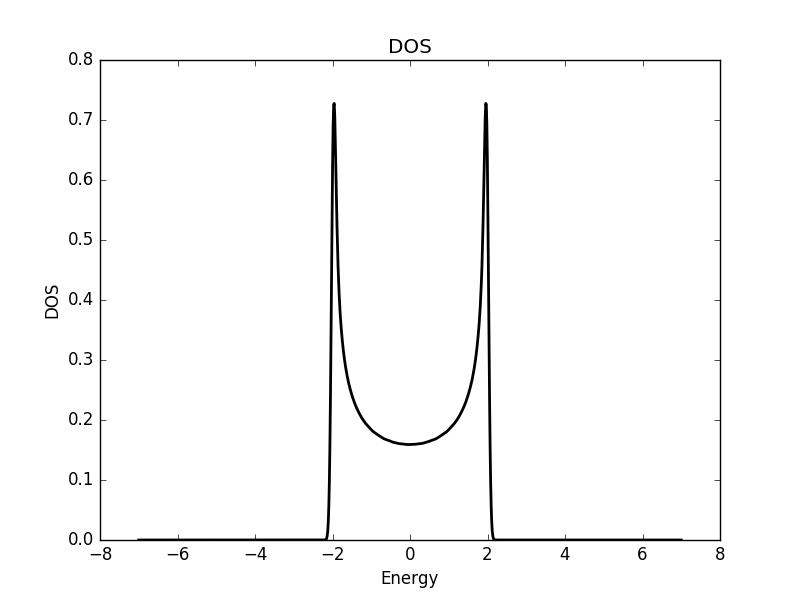
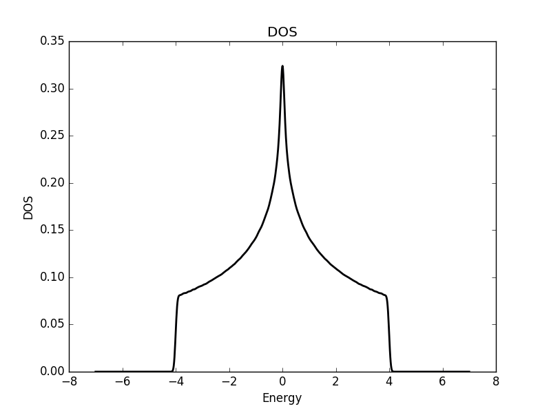
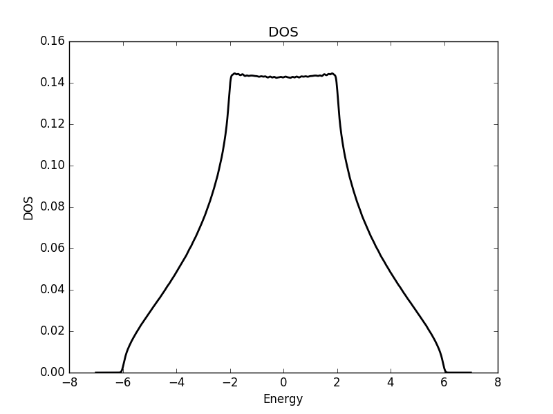
grid. value, we will use the Solver::BlockDiagonalizer. Knowing that the density of states will lie in the interval [-6, 6] for all three Models, we next setup the PropertyExtractor to work on the energy interval [-7, 7] and calculate the DOS. Finally we plot the DOS, using gaussian smoothin with
  and a convolution window of 101 energy points and save the results to file.