

Most recent TBTK release at the time of writing: v1.0.3
Updated to work with: v2.0.0
In this blog post we will take a look at how to specify models without necessarily knowing all the model parameters at the point of specification. This can be very useful when the Hamiltonian is time dependent or depends on some parameter that is to be solved for self-consistently.
We will here consider a third situation in which adjustable HoppingAmplitudes can be utilized by setting up a model with a variable potential. We will use this to repeatedly calculate the probability density and eigenvalues for the lowest energy states for seven different types of one-dimensional potentials. Namely, the infinite square well, square well, double square well, harmonic oscillator, double well, and step potential, as well as a potential with two regions with different potential separated by a barrier.
Parameters
The parameters that are needed are the number of sites to use for the discretized Schrödinger equation, the number of states for which we are going to calculate the probability density, and the nearest neighbor hopping amplitude  . We define these as follows.
//Number of sites and states to extract the
//probability density for.
const int SIZE_X = 500;
const int NUM_STATES = 7;
double t = 1;
We further create an enum that will be used to specify the type of the potential.
//Enum type for specifying the type of the
//potential.
enum PotentialType{
	InfiniteSquareWell,
	SquareWell,
	DoubleSquareWell,
	HarmonicOscillator,
	DoubleWell,
	Step,
	Barrier
};

//The type of the potential.
PotentialType potentialType;
Potential function
We also define a potential function that will be responsible for returning the potential at any given point.
//Function that dynamically returns the current potential on a given site.
complex<double> potential(int x){
	switch(potentialType){
	case InfiniteSquareWell:
		return infiniteSquareWell(x);
	case SquareWell:
		return squareWell(x);
	case DoubleSquareWell:
		return doubleSquareWell(x);
	case HarmonicOscillator:
		return harmonicOscillator(x);
	case DoubleWell:
		return doubleWell(x);
	case Step:
		return step(x);
	case Barrier:
		return barrier(x);
	default:
		Streams::out << "Error. This should never happen.";
		exit(1);
	}
}
Depending on the current potential type, this function calls one of several specific potential functions. The definition of these can be seen in the full source code linked at the end of this post.
Callback function
Normally a HoppingAmplitude is specified as
HoppingAmplitude(value, toIndex, formIndex);
However, it is also possible to pass a callback instead of a value as the first argument. This callback will later be called by the HoppingAmplitude to determine the value, passing the toIndex and fromIndex as arguments. That is, the HoppingAmplitude will “call back” later to determine the value.
For a class to classify as a valid callback function, it needs to inherit from HoppingAmplitude::AmplitudeCallback and provide a function that takes two indices as arguments and returns a complex value. In addition, it needs to be able to handle every pair of indices that it will be called with. That is, every pair of indices which it is packed together with into a HoppingAmplitude when the model is specified.
In this example, the position can be read off from either of the indices. In the following implementation, we read it off from the *from* Index and pass it to the potential function defined above to get the value for the potential.
//Callback that dynamically returns the current
//value on a given site.
class PotentialCallback : public HoppingAmplitude::AmplitudeCallback{
public:
	complex<double> getHoppingAmplitude(
		const Index &to,
		const Index &from
	){
		return potential(from[0]);
	}
} potentialCallback;
In the last line, we instantiate an object of the *PotentialCallback* called *potentialCallback*. It is this object that will be used as callback when specifying the model.
Model
The model that we will consider is the discretized one-dimensional Schrödinger equation which we specify as follows.1
//Create the Model.
Model model;
for(unsigned int x = 0; x < SIZE_X; x++){
	//Kinetic terms.
	model << HoppingAmplitude(
		2*t,
		{x},
		{x}
	);
	if(x + 1 < SIZE_X){
		model << HoppingAmplitude(
			-t,
			{x + 1},
			{x}
		) + HC;
	}

	//Potential term.
	model << HoppingAmplitude(
		potentialCallback,
		{x},
		{x}
	);
}
model.construct();
The kinetic terms result from discretizing the Laplace operator and letting  , while the potential term has been added by passing the callback *potentialCallback* as the first parameter to the HoppingAmplitude.
Set up the Solver and PropertyExtractor
We next set up the Solver and PropertyExtractor as follows.
//Setup the Solver and PropertyExtractor.
Solver::Diagonalizer solver;
solver.setModel(model);
PropertyExtractor::Diagonalizer
	propertyExtractor(solver);
The main loop
In the main loop, we will carry out the same calculation for each potential. We therefore begin by creating a list of potential types to perform the calculations for, and a list of filenames to which to save the results.
//List of potentials to run the calculation
//for.
vector<PotentialType> potentialTypes = {
	InfiniteSquareWell,
	SquareWell,
	DoubleSquareWell,
	HarmonicOscillator,
	DoubleWell,
	Step,
	Barrier
};

//List of filenames to save the results to.
vector<string> filenames = {
	"figures/InfiniteSquareWell.png",
	"figures/SquareWell.png",
	"figures/DoubleSquareWell.png",
	"figures/HarmonicOscillator.png",
	"figures/DoubleWell.png",
	"figures/Step.png",
	"figures/Barrier.png"
};
The main loop itself is as follows.
//Run the calculation and plot the result for
//each potential.
for(
	unsigned int n = 0;
	n < potentialTypes.size();
	n++
){
	//Set the current potential.
	potentialType = potentialTypes[n];

	//Run the solver.
	solver.run();

	//Calculate the probability density
	//for the first NUM_STATES.
	Array<double> probabilityDensities(
		{NUM_STATES, SIZE_X}
	);
	for(
		unsigned int state = 0;
		state < NUM_STATES;
		state++
	){
		for(
			unsigned int x = 0;
			x < (unsigned int)SIZE_X;
			x++
		){
			complex<double> amplitude
				= propertyExtractor.getAmplitude(
					state,
					{x}
				);
			probabilityDensities[{state, x}]
				= pow(abs(amplitude), 2);
		}
	}

	//Calculate the eigenvalues.
	Property::EigenValues eigenValues
		= propertyExtractor.getEigenValues();

	//Plot the results.
	plot(
		probabilityDensities,
		eigenValues,
		filenames[n]
	);
}
Here we loop over each type of potential and set the global parameter potentialType to the current potential in line 9. The solver is then executed, which results in the HoppingAmplitudes being requested internally, which triggers the callback functions to be called and return the values for the current potential. Next, the probability density is calculated2, followed by the calculation of the eigenvalues.
Finally, the results are plotted and saved to file. The plotting routine involves significant post processing of the data and the full code for achieving this can be found in the code linked below. In particular, the probability densities are first rescaled such that NUM_STATES probability densities can be stacked evenly on top of each other without overlapping or extending beyond the plotting window. Then the probability densities are shifted by the respective eigenvalue of the corresponding state to simultaneously convey information about the probability density and the eigenvalues in relation to the potential.
Results
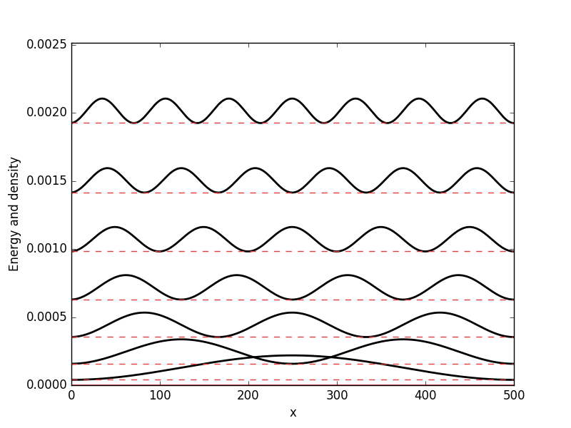
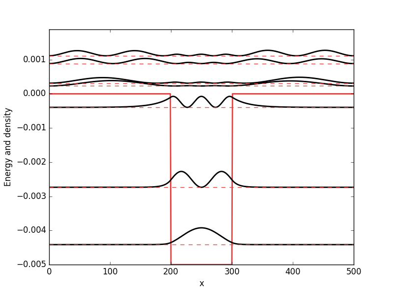
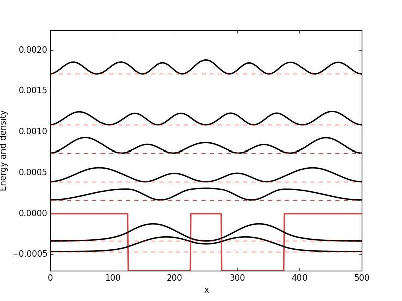
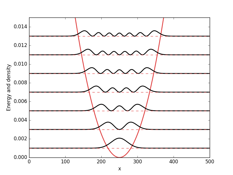
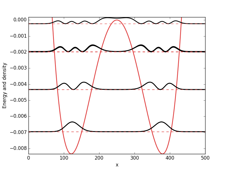
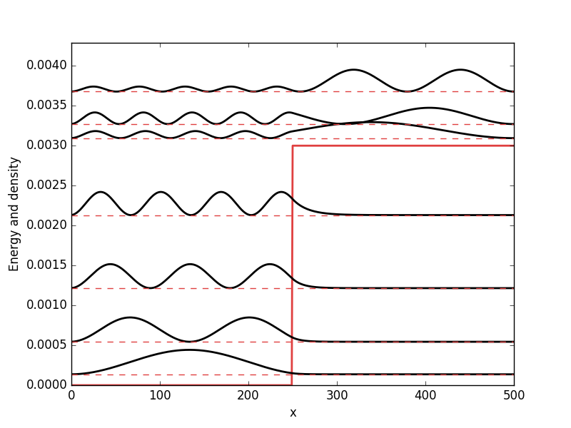
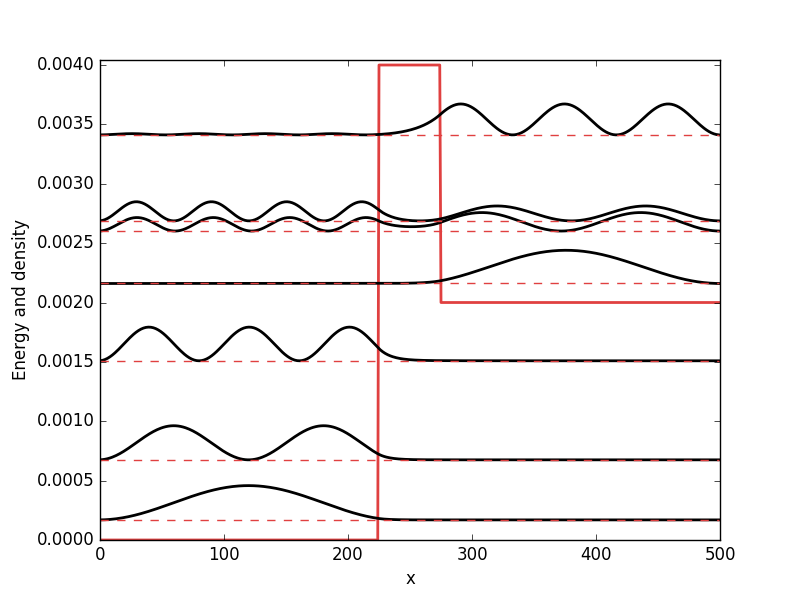
Below the results are presented. The thick red line indicates the potential, while the black lines are the probability densities. Each probability density has been offset by the corresponding states eigenvalue to put its energy in relation to the potential. The eigenvalues are also plotted with thin red lines. In agreement with the basic principles of quantum mechanics, we see how the states are oscillating in the regions where the potential is smaller than the energy of the state, while they decay exponentially into the regions where the potential is larger.
Infinite square well
Square well
Double square well
Harmonic oscillator
Double well
Step
Barrier
Full code
Full code is available in src/main.cpp in the project 2018_11_07 of the Second Tech code package. See the README for instructions on how to build and run.
- For more details see for example Using TBTK to calculate the density of states (DOS) of a 1D, 2D, and 3D square lattice and Direct access to wave function amplitudes and eigenvalues in TBTK
- See Direct access to wave function amplitudes and eigenvalues in TBTK for a more detailed description of the calculation of the probability density.