Using TBTK to calculate the density of states (DOS) of a 1D, 2D, and 3D square lattice

Most recent TBTK release at the time of writing: v1.0.2
Updated to work with: v2.0.0

In this post we will walk through how to calculate and plot the density of state (DOS) of a 1D, 2D, and 3D square lattice, using TBTK. To achieve this we will first implement three functions for creating the corresponding models. We will then create a fourth function in which the DOS is calculated for each of the three models.

This example also provides a simple demonstration of how TBTK naturally support the creation of general purpose code, in this case the calculation of the DOS, that can be used independently of the details of the model.

Creating the Model

One dimension

In one dimension the Hamiltonian is given by

$H_{1D} &= -2t\sum_{k_x}\cos(k_x)c_{k_x}^{\dagger}c_{k_x},$

where $t$ is a hopping parameter that we will set to one.

To create the model we loop over the summation index and feed each of the hopping amplitudes to the Model. Note how we let the numerical indices run over the positive discrete values 0 to 9999, while the argument of the cos function falls in the interval $[-\pi, \pi]$ .

Model createModel1D(){
    //Parameters.
    const int SIZE_X = 10000;
    double t = 1;

    //Create the Model.
    Model model;
    for(int kx = 0; kx < SIZE_X; kx++){
        double KX = 2*M_PI*kx/(double)SIZE_X - M_PI;
        model << HoppingAmplitude(
            -2*t*cos(KX),
            {kx},
            {kx}
        );
    }

    return model;
}

Two dimensions

In two dimension the Hamiltonian is given by

$H_{2D} &= -2t\sum_{k_x,k_y}\left(\cos(k_x) + \cos(k_y)\right)c_{\mathbf{k}}^{\dagger}c_{\mathbf{k}},$

where $\mathbf{k} = (k_x, k_y)$ .

The corresponding Model is created as follows using a $500\times 500$ grid.

Model createModel2D(){
    //Parameters.
    const int SIZE_X = 500;
    const int SIZE_Y = 500;
    double t = 1;

    //Create the Model.
    Model model;
    for(int kx = 0; kx < SIZE_X; kx++){
        for(int ky = 0; ky < SIZE_Y; ky++){
            double KX = 2*M_PI*kx/(double)SIZE_X;
            double KY = 2*M_PI*ky/(double)SIZE_Y;

            model << HoppingAmplitude(
                -2*t*(cos(KX) + cos(KY)),
                {kx, ky},
                {kx, ky}
            );
        }
    }

    return model;
}

Three dimensions

In three dimension the Hamiltonian is given by

$H_{3D} &= -2t\sum_{k_x,k_y,k_z}\left(\cos(k_x) + \cos(k_y) + \cos(k_z)\right)c_{\mathbf{k}}^{\dagger}c_{\mathbf{k}},$

where $\mathbf{k} = (k_x, k_y, k_z)$ .

The corresponding Model is created as follows using a $200\times 200\times 200$ grid.

Model createModel3D(){
    //Parameters.
    const int SIZE_X = 200;
    const int SIZE_Y = 200;
    const int SIZE_Z = 200;
    double t = 1;

    //Create the Model.
    Model model;
    for(int kx = 0; kx < SIZE_X; kx++){
        for(int ky = 0; ky < SIZE_Y; ky++){
            for(int ky = 0; ky < SIZE_Y; ky++){
                double KX = 2*M_PI*kx/(double)SIZE_X;
                double KY = 2*M_PI*ky/(double)SIZE_Y;
                double KZ = 2*M_PI*kz/(double)SIZE_Z;

                model << HoppingAmplitude(
                    -2*t*(cos(KX) + cos(KY) + cos(KZ)),
                    {kx, ky, kz},
                    {kx, ky, kz}
                );
            }
        }
    }

    return model;
}

Calculating the DOS

We are now ready to implement the main function for calculating the DOS. To take advantage of that the Hamiltonian consists of independent blocks for each $\mathbf{k}$ value, we will use the Solver::BlockDiagonalizer. Knowing that the density of states will lie in the interval [-6, 6] for all three Models, we next setup the PropertyExtractor to work on the energy interval [-7, 7] and calculate the DOS. Finally we plot the DOS, using gaussian smoothin with $\sigma = 0.05$ and a convolution window of 101 energy points and save the results to file.

int main(int argc){
    //Initialize TBTK.
    Initialize();

    //Filenames to save the figures as.
    string filenames[3] = {
        "figures/DOS_1D.png",
        "figures/DOS_2D.png",
        "figures/DOS_3D.png",
    };

    //Loop over 1D, 2D, and 3D.
    for(int n = 0; n < 3; n++){
        //Create the Model.
        Model model;
        switch(n){
        case 0:
            model = createModel1D();
            break;
        case 1:
            model = createModel2D();
            break;
        case 2:
            model = createModel3D();
            break;
        default:
            Streams::out << "Error: Invalid case value.\n";
            exit(1);
        }

        //Setup and run the Solver.
        Solver::BlockDiagonalizer solver;
        solver.setModel(model);
        solver.run();

        //Setup the PropertyExtractor.
        PropertyExtractor::BlockDiagonalizer propertyExtractor(solver);
        propertyExtractor.setEnergyWindow(-7, 7, 1000);
        Property::DOS dos = propertyExtractor.calculateDOS();

        //Normalize the DOS.
        for(unsigned int c = 0; c < dos.getResolution(); c++)
                dos(c) = dos(c)/model.getBasisSize();

        //Smooth the DOS.
        const double SMOOTHING_SIGMA = 0.05;
        const unsigned int SMOOTHING_WINDOW = 101;
        dos = Smooth::gaussian(dos, SMOOTHING_SIGMA, SMOOTHING_WINDOW);

        //Plot and save the result.
        Plotter plotter;
        plotter.plot(dos);
        plotter.save(filenames[n]);
    }

    return 0;
}

Results

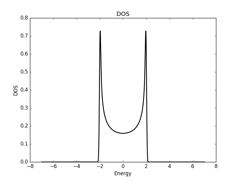
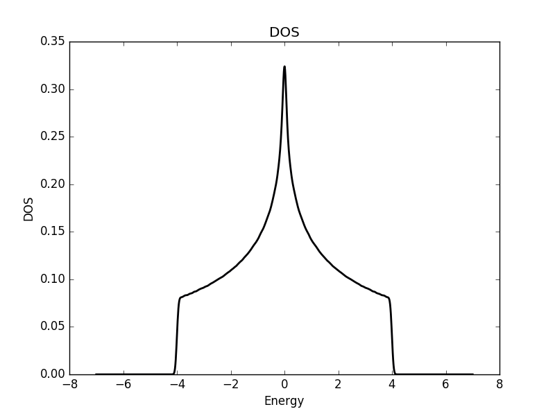
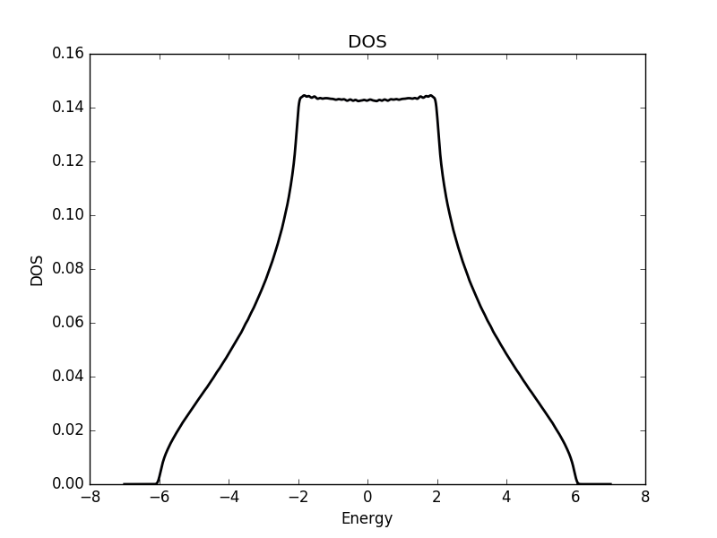
Below we show the result of the calculation for the three different cases.

One dimensional

Two dimensional

Three dimensional

Full code

Full code is available in src/main.cpp in the project 2018_10_23 of the Second Tech code package. See the README for instructions on how to build and run.