Direct access to wave function amplitudes and eigenvalues in TBTK

Most recent TBTK release at the time of writing: v1.0.3
Updated to work with: v2.0.0.

The wave functions and corresponding eigenvalues provide complete information about a system, from which other properties can be calculated. In this post we will therefore take a look at how to extract these directly using the Solver::Diagonalizer. In particular, we show how to calculate the energy and probability density for a given state in a two-dimensional rectangular geometry.

Model

The model that we will consider is a simple two-dimensional square lattice with nearest neighbor hopping $t = 1$ , for which the Hamiltonian is

$H = -t\sum_{\langle ij\rangle}c_{i}^{\dagger}c_{j}.$

Here $\langle ij\rangle$ denotes summation over nearest neighbors.

The Hamiltonian $H$ can either be viewed as the simplest example of a two-dimensional tight-binding model, or as a discretized version of the two-dimensional Schrödinger equation

$H_{S} = \frac{-\hbar^2}{2m}\left(\frac{\partial^2}{\partial x^2} + \frac{\partial^2}{\partial y^2}\right) + V(x,y),$

with $\hbar^2/2mdx^2 = \hbar^2/2mdy^2 = t$ and $V(x, y) = -4$ . We therefore begin by introducing the following parameters.

//Parameters.
const unsigned int SIZE_X = 20;
const unsigned int SIZE_Y = 20;
double t = 1;
int state = 0;

The last parameter is used to indicate for which state we are going to calculate the energy and probability density.

We next create the model and loop over each site to feed the model with the hopping amplitudes. We could achieve this by for each site adding the hopping amplitudes corresponding to

$\begin{aligned} -t&\left(c_{(x+1,y)}^{\dagger}c_{(x,y)} + c_{(x-1,y)}^{\dagger}c_{(x,y)}\right.\\ &+\left.c_{(x,y+1)}^{\dagger}c_{(x,y)} + c_{(x,y-1)}^{\dagger}c_{(x,y)}\right). \end{aligned}$

However, we note that this is equivalent to adding

$-t\left(c_{(x+1,y)}^{\dagger}c_{(x,y)} + c_{(x,y+1)}^{\dagger}c_{(x,y)}\right) + H.c.$

at each site since for example $-tc_{(x-1,y)}^{\dagger}c_{(x,y)}$ is the Hermitian conjugate of $-tc_{(x,y)}^{\dagger}c_{(x-1,y)}$ .¹ Using the later notation we implement this as follows.

//Create the Model.
Model model;
for(unsigned int x = 0; x < SIZE_X; x++){
	for(unsigned int y = 0; y < SIZE_Y; y++){
		if(x+1 < SIZE_X){
			model <<; HoppingAmplitude(
				-t,
				{x + 1, y},
				{x,     y}
			) + HC;
		}
		if(y+1 < SIZE_Y){
			model << HoppingAmplitude(
				-t,
				{x, y + 1},
				{x, y}
			) + HC;
		}
	}
}
model.construct();

The if statements are added to guard against adding hopping amplitudes beyond the boundary of the system.

Solver

We are now ready to setup and run the solver.

//Setup and run the Solver.
Solver::Diagonalizer solver;
solver.setModel(model);
solver.run();

Extract the eigenvalue and probability density

To extract the eigenvalue and probability density we first setup the PropertyExtractor.

//Setup the PropertyExtractor.
PropertyExtractor::Diagonalizer
    propertyExtractor(solver);

After this we print the energy for the given state by requesting it from the PropertyExtractor.

//Print the eigenvalue for the given state.
Streams::out << "The energy of state "
    << state << " is "
    << propertyExtractor.getEigenValue(state)
    << "\n";

Further, to calculate the probability density we create an array, which we fill with the square of the absolute value of the probability amplitude.

//Calculate the probability density for the
//given state.
Array<double> probabilityDensity(
    {SIZE_X, SIZE_Y}
);
for(unsigned int x = 0; x < SIZE_X; x++){
	for(unsigned int y = 0; y < SIZE_Y; y++){
		//Get the probability amplitude at
		//site (x, y) for the given state.
		complex<double> amplitude
			= propertyExtractor.getAmplitude(
				state,
				{x, y}
			);

		//Calculate the probability density.
		probabilityDensity[{x, y}] = pow(
			abs(amplitude),
			2
		);
	}
}

Finally, we plot the probability density and save it to file.

//Plot the probability density.
Plotter plotter;
plotter.plot(probabilityDensity);
plotter.save("figures/ProbabilityDensity.png");

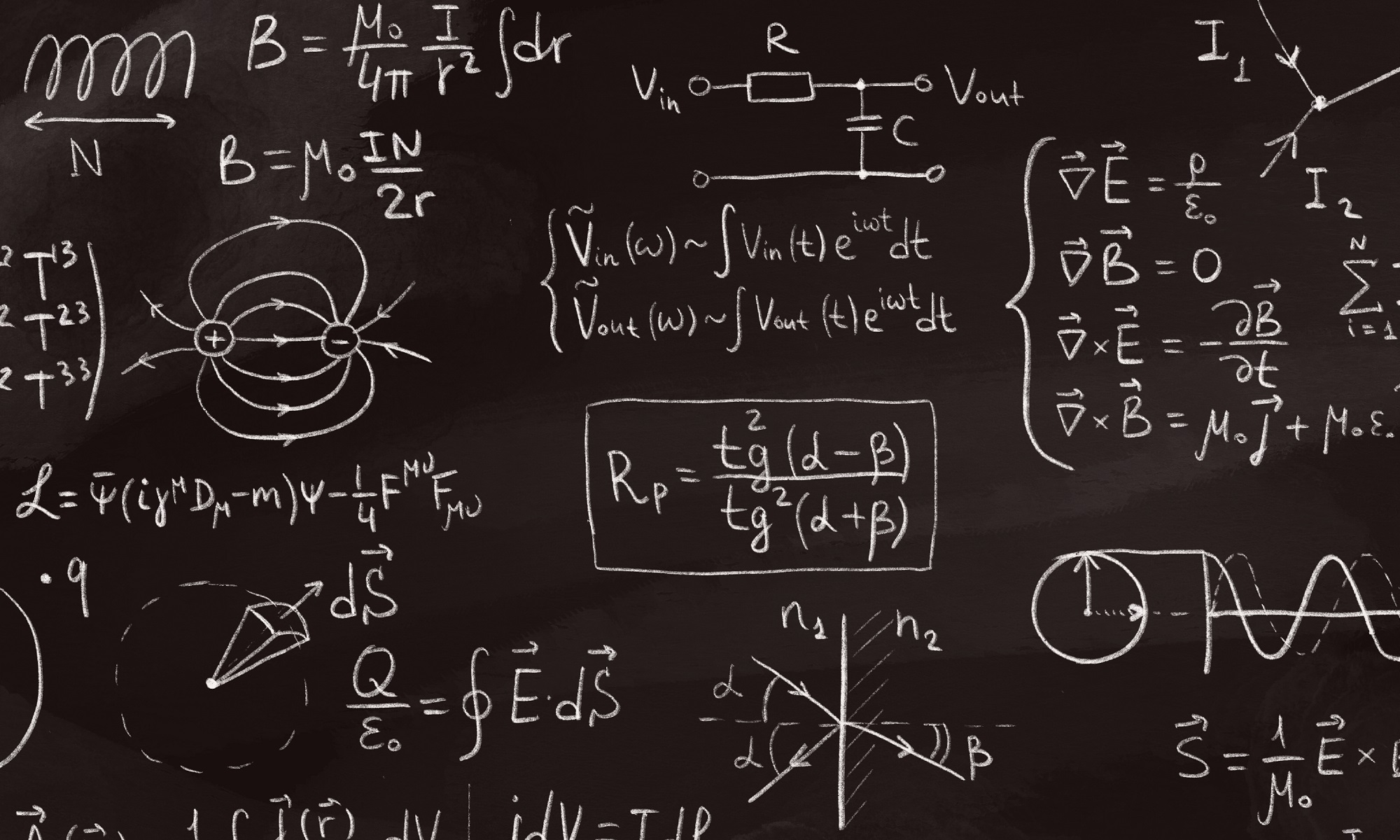
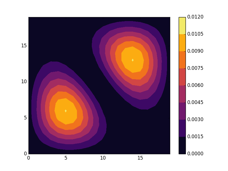
Results

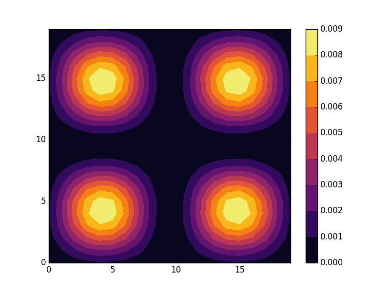
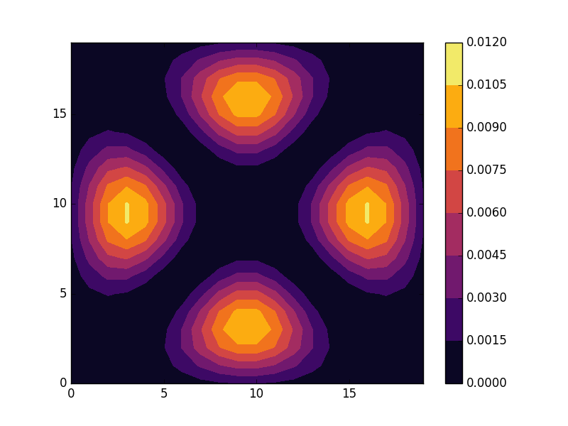
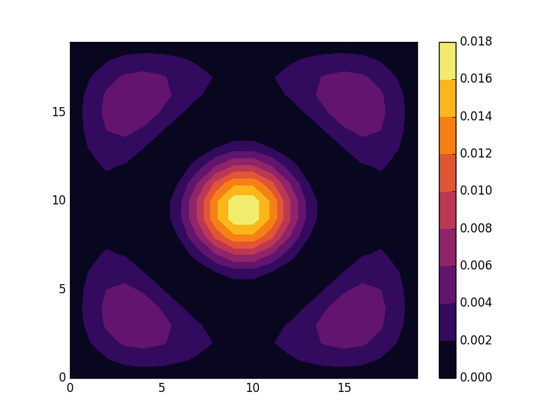
Below we present the results for the six lowest energy states for a lattice size of 20×20. The states separate into four groups with eigenvalues

$E \in \{-3.9553, -3.8881, -3.82229, -3.7796\}.$

The second and fourth of these eigenvalues are degenerate with two eigenfunctions per energy. We can understand this grouping by realizing that the solutions to our problem are sinus functions with wave numbers (m, n),² where for the six lowest states

$(m, n) \in \{(1, 1), (2, 1), (1, 2), (2, 2), (3, 1), (1, 3)\}.$

Among these (2,1) and (1, 2) as well as (3, 1) and (1, 3) are degenerate.

E = -3.9553

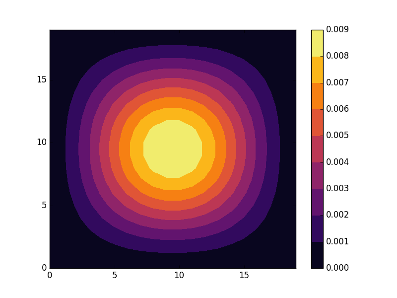
E = -3.88881 (two degenerate states)

E = -3.82229

E = -3.7796 (two degenerate states)

Full code

Full code is available in src/main.cpp in the project 2018_10_27 of the Second Tech code package. See the README for instructions on how to build and run.

Note that the two expressions are not equivalent on each individual site since the Hermitian conjugate of one term is a term that appears in the former expression on a different site. The two prescriptions are only equivalent since we add the terms on all sites.
This is most easily understood from considering the continous Schrödinger equation above, but is also true for the discrete lattice.