
Most recent TBTK release at the time of writing: v1.0.3
Updated to work with: v2.0.0
One of the core strengths of TBTK is the generality of the quantum systems that can be modeled and the ease with which such models can be created. In this post we will take a look at how the use of an IndexFilter can simplify this process further. In particular, we will show how to setup the Schrödinger equation on a simple annulus shaped geometry and how to calculate the energy and probability density for a given state.
In addition to showing how to use an IndexFilter, this post also provides a simple example of quantum mechanics in polar coordinates. The solutions we arrive at show similarities with the s, p, and d orbitals, and the radial wave functions that appears as solutions to the Schrödinger equation in a central potential (the Hydrogen atom). This without the need of introducing a spatially varying potential. As such it can give useful insights into aspects of quantum mechanics that can be difficult to grasp from the derivation of the solutions to the full fledged Schrödinger equation in a central potential.
The material closely parallels the earlier post Direct access to wave function amplitudes and eigenvalues in TBTK, which provide more details on some of the content that is treated more briefly here.
Model
The model that we consider here is the Hamiltonian
![\[ H = -t\sum_{\langle ij\rangle}c_{i}^{\dagger}c_{j}, \]](https://second-tech.com/wordpress/wp-content/ql-cache/quicklatex.com-8192fbef0d654403e8bd881d74741a3a_l3.png "Rendered by QuickLaTeX.com")
on an annulus with inner radius  and outer radius
  . Here
  denotes summation over nearest neighbors and the Hamiltonian can be considered to be the (square lattice) discretized version of the Schrödinger equation with
![\[\begin{aligned} H_{S} &= \frac{-\hbar^2}{2m}\left(\frac{\partial^2}{\partial x^2} + \frac{\partial^2}{\partial y^2}\right) + V(x,y)\\ &= \frac{-\hbar^2}{2m}\left(\frac{1}{r}\frac{\partial}{\partial r}\left(r\frac{\partial}{\partial r}\right) + \frac{1}{r^2}\frac{\partial^2}{\partial \theta^2}\right) + V(r, \theta), \end{aligned}\]](https://second-tech.com/wordpress/wp-content/ql-cache/quicklatex.com-792d9a388f86a4b5574a9d21ca16cb5d_l3.png "Rendered by QuickLaTeX.com")
with  and
and  .
.
Parameters
To set up this model we first specify the following parameters.
//Parameters.
const unsigned int SIZE = 41;
const unsigned int SIZE_X = SIZE;
const unsigned int SIZE_Y = SIZE;
const double OUTER_RADIUS = SIZE/2;
const double INNER_RADIUS = SIZE/8;
double t = 1;
int state = 0;
The first three parameters specifies an underlying  grid. The fourth and fifth parameter defines the outer and inner radius of the annulus and we also set
  . The last parameter is used to indicate for which state we are going to calculate the energy and probability density.
IndexFilter
The basic idea behind an IndexFilter is to allow for geometry specific information to be separated from the specification of the Hamiltonian.
It is possible to add if-statements in the model specification to guard against the addition of HoppingAmplitudes to sites that are not supposed to be included. However, allowing for such elements to be passed to the Model and instead use a filter to exclude invalid terms results in cleaner and less error prone code.
To create an IndexFilter we need to inherit from the class AbstractIndexFilter and implement the functions clone() and isIncluded().
//IndexFilter.
class MyIndexFilter
	: public AbstractIndexFilter{
public:
	//Implements AbstractIndexFilter::clone().
	MyIndexFilter* clone() const{
		return new MyIndexFilter();
	}

	//Implements
	//AbstractIndexFilter::isIncluded().
	bool isIncluded(const Index &index) const{
		//Extract x and y from the Index.
		int x = index[0];
		int y = index[1];

		//Calculate the distance from the
		//center.
		double r = sqrt(
			pow(abs(x - (int)SIZE_X/2), 2)
			+ pow(abs(y - (int)SIZE_Y/2), 2)
		);

		//Return true if the distance is less
		//than the outer radius of the annulus,
		//but larger than the inner radius.
		if(r < OUTER_RADIUS && r > INNER_RADIUS)
			return true;
		else
			return false;
	}
};
For all basic use cases clone() can be implemented as above and we will therefore leave this function without further comments.
The first thing to note about isIncluded() is that it needs to be ready to accept any Index that is passed to the Model and return true or false depending on whether the Index is included or not. This means that the filter writer needs to be aware what type of indices that can be expected to be added to the model. In our case this is simple, our indices will all be of the form {x, y}. We can therefore immediately read of the x and y value from the first and second subindex. The distance  from the center of the grid is then calculated and true is returned if
  .
.
Create the Model
Having created the IndexFilter we are now ready to set up the actual model.
	//Create filter.
	MyIndexFilter filter;

	//Create the Model.
	Model model;
	model.setFilter(filter);
	for(unsigned int x = 0; x < SIZE_X; x++){
		for(unsigned int y = 0; y < SIZE_Y; y++){
			model << HoppingAmplitude(
				-t,
				{x + 1,	y},
				{x,     y}
			) + HC;
			model << HoppingAmplitude(
				-t,
				{x, y + 1},
				{x, y}
			) + HC;
		}
	}
	model.construct();
Compare this to the model creation in Direct access to wave function amplitudes and eigenvalues in TBTK. The first difference is the creation of the filter in the second line and the addition of this filter to the Model in the sixth line. Other than this the only difference is the absence of if-statements inside the loop. By using an IndexFilter we have made the annulus even simpler to setup than the square grid!
Solver
We are now ready to set up and run the solver.
//Setup and run the Solver.
Solver::Diagonalizer solver;
solver.setModel(model);
solver.run();
Extract the eigenvalue probability density
The code for extracting the eigenvalue (energy) and probability density and writing this to file is almost identical to the code in Direct access to wave function amplitudes and eigenvalues in TBTK.
//Setup the PropertyExtractor.
PropertyExtractor::Diagonalizer
	propertyExtractor(solver);

//Print the eigenvalue for the given state.
Streams::out << "The energy of state "
	<< state << " is "
	<< propertyExtractor.getEigenValue(state)
	<< "\n";

//Calculate the probability density for the
//given state.
Array<double> probabilityDensity(
	{SIZE_X, SIZE_Y},
	0
);
for(unsigned int x = 0; x < SIZE_X; x++){
	for(unsigned int y = 0; y < SIZE_Y; y++){
		if(!filter.isIncluded({x, y}))
			continue;
		//Get the probability amplitude at
		//site (x, y) for the
		//given state.
		complex<double> amplitude
			= propertyExtractor.getAmplitude(
				state,
				{x, y}
			);

		//Calculate the probability density.
		probabilityDensity[{x, y}] = pow(
			abs(amplitude),
			2
		);
	}
}

//Plot the probability density.
Plotter plotter;
plotter.plot(probabilityDensity);
plotter.save("figures/ProbabilityDensity.png");
There are only two minor difference, of which the first is the zero as second argument in the expression
Array<double> probabilityDensity(
	{SIZE_X, SIZE_Y},
	0
);
This is used to initialize every element to zero to make sure that elements outside of the annulus are not left uninitialized. The second difference is the appearance of the following two lines inside the loop.
if(!filter.isIncluded({x, y}))
	continue;
Here the IndexFilter is used once more to check whether a given Index is included in the Model or not. If not, we skip the rest of the loop body for this particular Index to avoid requesting data that does not exist.
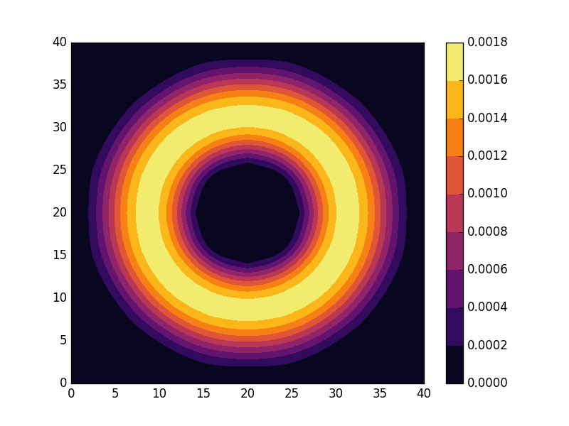
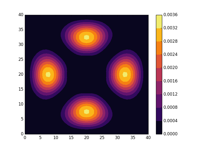
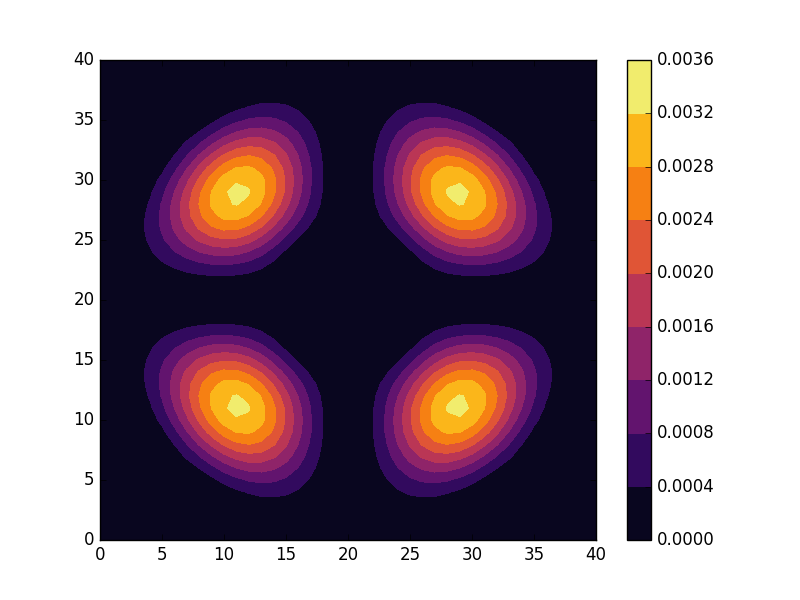
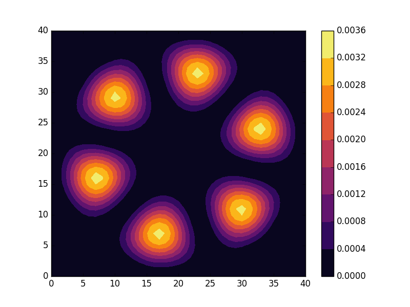
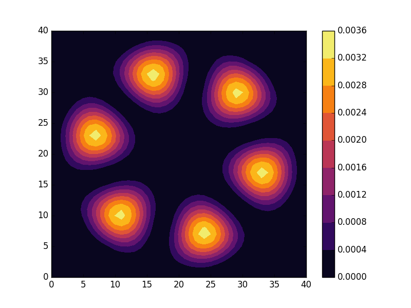
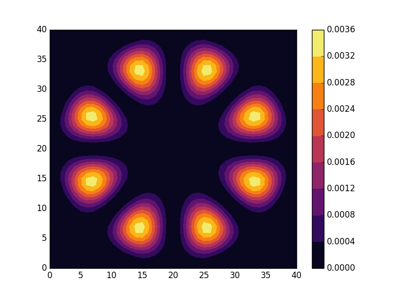
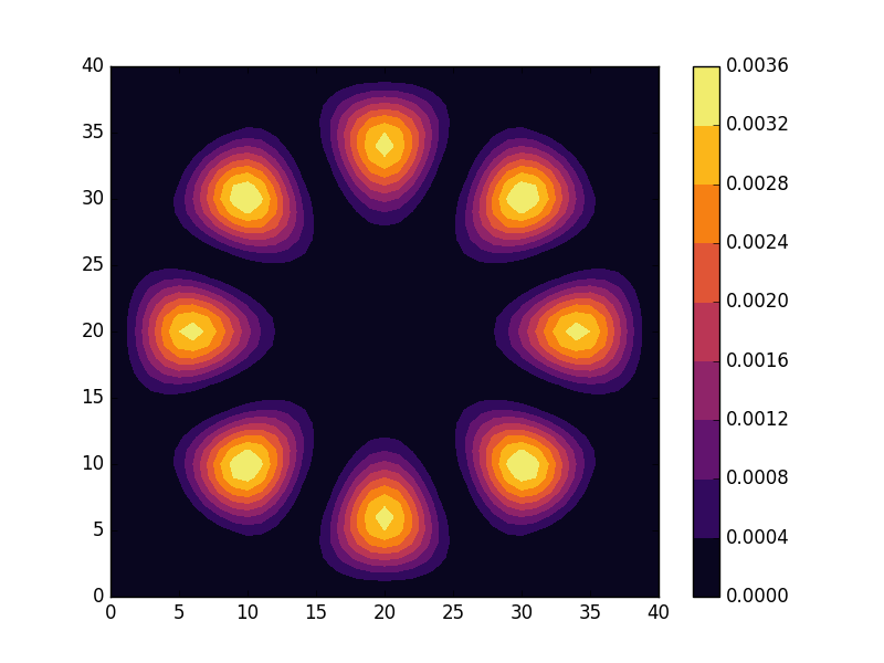
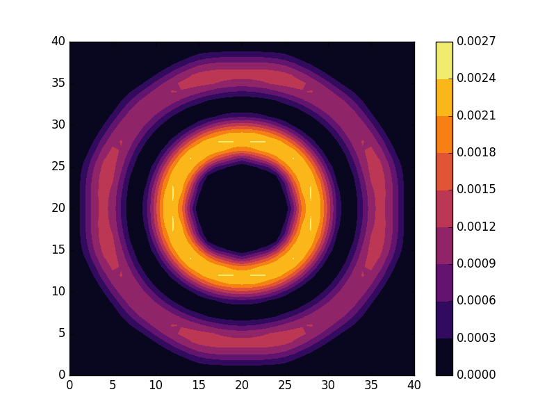
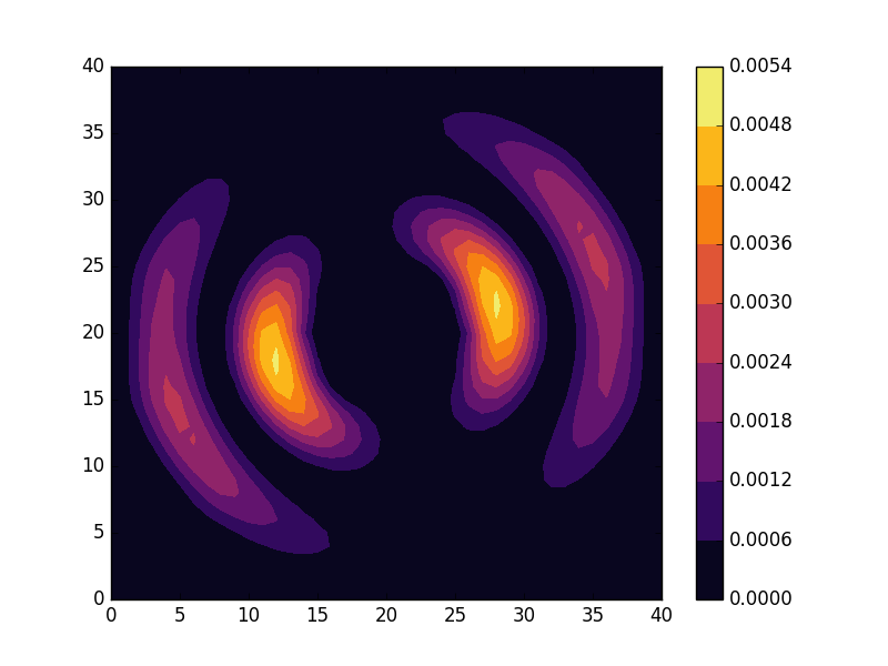
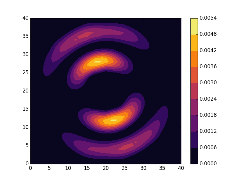
Results
Below we present the energies and probability densities for the eleven first states.


To understand these results we note that through separation of variables, the polar form of  can be seen to be solved by a function of the form
![\[ f_{n,m}(r, \theta) = f_{n}(r)e^{im\theta}. \]](https://second-tech.com/wordpress/wp-content/ql-cache/quicklatex.com-57f089d025846d33510057ced248434a_l3.png "Rendered by QuickLaTeX.com")
Here the radial function needs to satisfy the boundary conditions  . Moreover, it can be verified by application of
  to
to  that
that  and
and  are solutions with the same energy. In the continuous case we therefore expect non-degenerate eigenvalues for
  and doubly degenerate eigenvalues for
  . For the radial solutions we can further expect a set of increasingly oscillating functions with increasing
  .
.
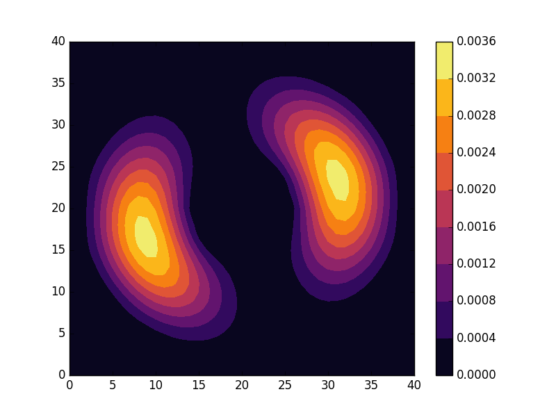
The numerical results are indeed in agreement with this observation. The 0th state displays a simple structure with a single radial oscillation and . State 1-8 appear in pairs with increasing wave number  along the
  direction. After state 8 it is no longer energetically favorable to keep increasing the angular wave number, but instead the next energy state is found by once again returning to the non-degenerate case
  , but to increase the radial wave number by one. This is then followed by another set of degenerate states with two radial oscillations and
  .
.
These observations are only approximate though, which we realize by noting that the probability density  actually is a constant function of for all . To understand why we see oscillations also in the probability density, we first note that
![\[ &\frac{1}{\sqrt{2}}\left(f_{n,m}(r, \theta) + f_{n,-m}(r, \theta)\right) = \sqrt{2}f_{n}(r)\cos(im\theta) \]](https://second-tech.com/wordpress/wp-content/ql-cache/quicklatex.com-1784965f8d2ceacd7e1c3e5026aa796a_l3.png "Rendered by QuickLaTeX.com")
and
![\[ &\frac{1}{\sqrt{2}}\left(f_{n,m}(r, \theta) + f_{n,-m}(r, \theta)\right) = \sqrt{2}if_{n}(r)\sin(im\theta) \]](https://second-tech.com/wordpress/wp-content/ql-cache/quicklatex.com-8bda533be7e972840f96ec5a69e40f3c_l3.png "Rendered by QuickLaTeX.com")
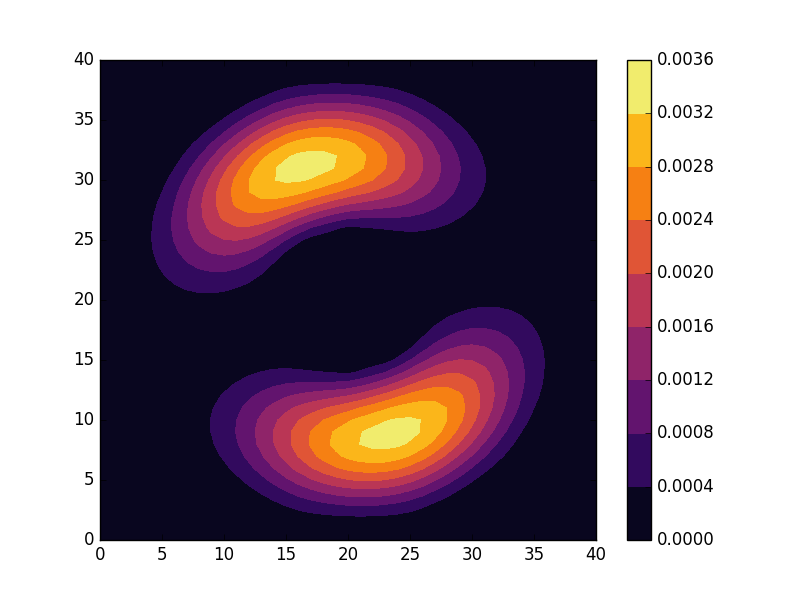
are equally valid eigenstates and display the spatial variation also for the probability density. Moreover, the degeneracy is only approximate in the discrete case, resulting in the true eigenstates resembling the later set more closely. Why the spatially modulated functions are preferred once the degeneracy is lifted can likely be understood by considering that spatial modulation allows the wave function of the lower energy state to avoid the areas that result in an increasing energy.
We finally note how the geometry of the problem results in solutions that naturally separate into a radial wave function multiplied by an angular wave function. This is in analogy with the solutions to the Schrödinger equation in a central potential, which gives rise to a separation between orbital and radial wave functions with independent wave numbers. However, in two dimensions the angular wave functions appear with a single non-degenerate solution followed by pairs of degenerate solutions (1, 2, 2, 2, …). In contrast, the spherical harmonics has two angular coordinates and the s, p, d, orbitals etc. instead has the degeneracies (1, 3, 5, …). First considering this simpler manifestation of this phenomenon can be useful to get a better understanding also of the solutions to the Schrödinger equation for the Hydrogen atom.
Full code
Full code is available in src/main.cpp in the project 2018_11_01 of the Second Tech code package. See the README for instructions on how to build and run.